ISSN: 1204-5357
ISSN: 1204-5357
Raymond Trémolières, Docteur es Sciences
Professor, Institut d'Etudes Politiques, Science-Po and FEA, Paul Cezanne University Aix en Provence, France
IEP, 25 rye Gaston de Saporta, F-13100 Aix en Provence.
Author's Personal/Organizational Website: www.credocom.fr, www.sciencespo.aix
Email: rtremolieres@cetfi.org
Prof. Raymond TREMOLIERES is the Director of AFERIA, Association Française d'Etudes et de Recherches en Intelligence Artificielle, His areas of interest are Finance, Technical and Quantitative Management, Data Analysis,Optimisation
Anton Turko, Docteur en Sciences de Gestion
Research Associate, FEA, CETFI, and Science-Po-Aix, University of Paul Cezanne , Aix en Provence
27 rue du petit puits, Marseille, 13002 France
Author's Personal/Organizational Website: www.credocom.fr, www.sciencespo.aix
Email: antturko@yahoo.fr
Dr. Anton TURKO is a Research Associate, FEA, CETFI, and Science-Po-Aix, University of Paul Cezanne, Aix en Provence, France. His current research interests are Finance, Derivatives, and Options Market.
Visit for more related articles at Journal of Internet Banking and Commerce
This paper follows a preceding paper by TREMOLIERES, TURKO, KARAM (2006) in which was proposed a specific behavioral model revealing the functioning of option markets and the way equilibrium values can be observed. We shall make use of Utility theory and Stochastic dominance. This model was illustrated earlier on simplified financial data. But our aim was to conduct a more realistic experimentation to reveal the logical probability function of market values. We build an information system using option market data available on internet. It is the purpose of the present paper to propose a new tool to analyze the financial market probability structure.
‘open-source’ database, financial markets, conditional markets, option markets, equilibrium prices, probability, derivatives, Market Probability Indicator.
An old model of one of the authors was first proposed in the context of ‘French prime markets’ which is here readapted to option markets. Here we give some new view points on the way equilibrium can exist and how the obtained underlying information can be used to forecast market prices. This comes from an in depth study on the way operators behave and how and when they express their knowledge of possible future probabilistic tendencies through available daily published data.
It is important to say that this model is not interested into sole pricing of stocks neither of options, contrary to the models of BACHELIER ( 1900), BLACK, SCHOLES (1973), COX (1985), BRENNAN, SCHWARTZ (1979) and so many others relying on efficient market assumptions.
Here we to introduce a new indicator called ‘MPI’. An application on French option market illustrates the way probabilistic forecasting can be implemented to predict market tendencies. This model makes use of available data bases that can be exploited freely on internet by professional's investors and academic people.
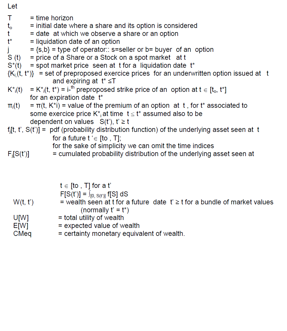
The model leads to use the following formulas where we consider shares priced not only on a ‘stock market’ but also on an option ‘conditional’ market. Two opposite operators, a seller and a buyer, intervene and interact on these markets and have normally different view points on price evolution.
We assume rational behaviors of sellers and buyers in order to predict market prices trends.
The model relies on the main following hypotheses:
H(1): at any t ∈ [to , T] , each operator has his own probability distribution (subjective) of the spot price for some t’ ≥ t, (normally t’ = t* op }
fj[S(t’), t, t’] , t ≤ t’ ∈ [to, T], j = {s,b}
where the parameters s , b, stand for ‘sellers’ and ‘buyers’. In the case of European Options, operators are essentially interested by t’= t*op .
H(2): Each operator is assumed to have a subjective rational behavior. The preferences of the operators are assumed to correspond to an utility function of their wealth seen at t’ from t
Uj [Wj (t, t’)] , t, t’ ∈ [to, T], j = {s,b} .
They seek to maximize their expected utility:
Max Ej [Uj [Wj (.)]] , j = {s,b}
H(3): All decisions take place in a limited time interval [to, T].
The expected value of wealth is
E[Wj (.)] = ∫[0, ∞] Wj (S) fj (S) dS
(not confound the function S(t) and the mute variable S).
The certainty monetary equivalent CMeq of the utility of wealth is obtained as the implicit value
Uj [CMeq [Wj (.)]] = ∫[0, ∞] Uj [Wj (S)] fj (S) dS
so
CMeq[Wj (.) = E[Wj (.)] + ej [Wj (.)], j = {s,b}
where ej ≤ 0 if the operator is risk averse and ej > 0 otherwise, j = {s,b}.
Different decisions are possible for the opposed operators j = {s,b.
Seller decision
Assuming that a seller owns some share at an initial time to , his initial wealth (we omit j) is
Wo = So = spot price at time to .
At any t ∈ [to, T], he can decide:
-.to keep his security on the spot market until t’≤ T then his wealth is
W(t, t’) = S(t’) ,
so we have
E[W(t, t’)] = E[S(t’)] = ∫[0, ∞] S f (S) dS ,
-.to sell the security on the future market, at some t = t*fut then is wealth is ‘certain’:
W~(t, t*)= S~(t, t*) = S*(t)
where ‘~’ stands for the future price S*. It is in reality a random variable at t < T, but because t is a ‘today’ value (when t = T or just before) it can be considered as a ‘quasi-certain’ or ‘quasi-deterministic’ random value. Furthermore one can also say that we have
E[W(t, t*)] = S*~(t, t*) which is the ‘quasi certain’ value of the day
.-to sell the security on the option market at some time t ≤ t*op then his wealth is given by
(1) W[t, t*] = S*(t) + π(t), if S(t*) ≤ K(t, t*)
(2) W[t, t*] = K(t, t*) + π(t) , if S(t*) ≥ K(t, t*) So
E[W(t, t*)] = ∫[0,K(t, t*)] [S + π(t)] f(S) dS + ∫[K(t,, t*), ∞] [K(t, t*) + π(t)] f(S) dS
hence
(3) E[W(t, t*)] = π(t) + ∫[0,K(t, t*)] S f(S) dS + ∫[K(t,, t*), ∞] K(t, t*) f(S) dS .
One can note that for the seller
(4) E[S*] ≤ E[W(t, t*)] ≤ π(t) + E[S*] .
Buyer decision
Here the decision of investing on future markets is let aside because of its less interest (leverage effect and unlimited possible losses), compared to the option markets, as shown in ancient papers on one of the author.
When we assume that the buyer initial wealth is
W0 = π = forfeit (or prime).
So the buyer can take one of the following decisions at any t ∈ [to, T] :
-keep his capital: then
W(t) = π(t), for any t ∈ [to, T]
E[W(t)] = π(t)
-buy on the option market (and resell) then
(5) W(t, t*) = π(t) – π(t) = 0, if S(t*) ≤ K(t, t*)
(6) W(t, t*) = S(t*) – [K(t, t*) + π(t)] if S(t*) ≥ K(t, t*).
In this case, the buyer expected value of a call option is
(7) E[W(t, t*)] = ∫[K(t, t*), ∞] (S – [K(t, t*)+ π(t)]) f(S) dS
Rational decision criteria
Set
es , eb = risk parameters for a seller and a buyer.
From the above mentioned assumptions (3), (7) we can write the rational decision criteria of both operators at any time t ∈ [to, T]
-.for the seller: sell on the option market if:
(8) (K + π) [1-F(K)] +∫[0, K] (S + π) f(S) dS ≥ S* + es
(9) π + ∫[0, K] S f(S) dS + K [1-F(K)] ≥ S* + es
-.for the buyer: buy on the option market if
(10) ∫[K,∞] [S-(K+ π)] f(S) dS ≥ π + eb
(11) ∫ [K,∞] S f(S) dS - (K + π) [1 – F(K)] ≥ π + eb
In order that the operators agree to go on the option market for a transaction, then the two inequations must be satisfied for both of them but not necessarily with the same pdf.
It is easy to check that the price slack
X(t) – S*(t) = K(t) + π(t) – S*(t)
is related to f(S) for the seller. This leads to deduce that (8) can be transposed as a forecasting tool. Indeed, because K, π and S*(t) are known over past periods it is possible to get information on f(S) and its changes.
In the case of several values of K, π , available the same day, all these data can be exploited to elaborate information on f(S).
We make use of (8) and (10) to obtain relationships between K, π , S*(t), F(.) .
Consider
-two different dates t and t’ (t < t’)
-or two distinct quotations (i,t) , (i',t') at a same date or even for two different dates
and set
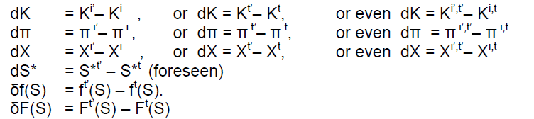
(it is also possible to consider that f, F varies along with quotations)
Here one can also use δX = Xt’,i' – Xt,i , δS* = S*t’,i' – S*t,i , but we prefer to draw the attention on discrete changes in the probabilities that could be better seen on more than one day variation.
Seller relationship
By second order stochastic dominance considerations (as done in our first articles on ‘prime’ markets) or simply, using the expected value criterion and assuming (8) as an equality we obtain:
(12) π + ∫[0, K(t)] S f(t, S) dS + K [1- F(t, K(t))] = S*(t) .
Everything being equal and assuming some correlative variation of X=K+π , dX=dK+dπ , and dS* one can differentiate with respect to time (one can subtracts (8) at any t from the same equality at any t’> t and develop at the first order we get
(13) dπ + dK{1 – F[K + dK] - δF[K + dK]} – π δF(K) –
-K{F[K + dK] – F(K ) + δF[K + dK]} +
+ ∫[K, K +dK] S f(S) dS + ∫[0, K +dK] S δf(S) dS = dS* .
This formula must not be applied as it is and should be simplified according to cases.
For example, assuming that the pdf doesn’t vary then one obtains:
(14) dπ + dK[1 – F(K + dK)] – K [F(K + dK) – F(K)] + ∫[K, K +dK] S f(S) dS = dS* ,
which can be simplified again, for example, assuming dK small for the integrated terms one has
(15) dπ + dK [1 – F(K)] + ∫[K, K +dK] S f(S) dS = dS* ,
and finally
(16) dπ + dK [1 – F(K)] = dS* , (or ≤ dS*) .
Observe that in this case, dS* must be normally close to zero if the anticipation of an unchanged probability distribution is correct, thus in the non changing case, an approximate formula will be
(17) dπ + dK [1 – F(K)] = 0 , (or ≤ 0) ,
or
(18) dK/dπ = - 1/ [1 – F(K)] .
A very well known negative relationship between π and K is shown here; also
(19) F(S=K) = 1 + dπ/dK
Here we choose to emphasize the Seller point of view (the one of the buyer is presented in (TREMOLIERES, TURKO (2009)).
From (19) we can exhibit F(S*) and obtain the Market Probability Indicator MPI, as shown in the following table.
On February 3 , 2006, the characteristics of pair {exercice price, pemium} for a Call on France Telecom expiring Sept 2009 are given in Table.1

Table.1: Details of the computation of MPI compared to price S(t).

Figure. 2: Dayly Spot price of France Telecom Stock [Mai03-Mai09].

Figure. 3: MPI calculated with call option prices of France Telecom [Mai03-Mai09].
Note that tne MPI variations are generally opposed to the market trends.
In what precedes, the MPI has been represented as a set of several curves (like a 'comb') stopping at several expiration dates and gives information on the possible In what precedes, the MPI has been represented as a set of several curves (like a 'comb') stopping at several expiration dates and gives information on the possible probabilistic evolution of the market. Data where directly taken from internet where data can be obtained freely from EuroNext. A time lag of 15 minutes is however necessary to catch most of the traders subjective probabilities.
Copyright © 2026 Research and Reviews, All Rights Reserved