MODELING OF THE ECONOMIC CYCLES USING THE THEORY OF FRACTIONAL CALCULUS

Vitus Bering Kamchatka State University, Petropavlovsk-Kamchatskiy, Pogranichnaya, Russia

Vitus Bering Kamchatka State University, Petropavlovsk-Kamchatskiy, Pogranichnaya, Russia

*Corresponding Author:

Danil Vasilevich Makarov
Vitus Bering Kamchatka State University
Petropavlovsk-Kamchatskiy
Pogranichnaya, Russia
Tel: + 8 (4152) 42-68-42
E-mail: danil.makarov.asu@bk.ru

Visit for more related articles at Journal of Internet Banking and Commerce

Abstract

This paper presents a mathematical model that generalizes the famous Kondratiev cycles model (Dubovskiy model) used to predict economic crises. This generalization is to integrate the memory effect, which occurs frequently in the economic system. With the help of numerical methods, a generalized model was received, according to which the phase paths were built.

Keywords

Kondratiev Cycles, Economic Crisis, Dubovskiy Model, Gerasimov-Caputo Fractional Derivative Operator, Memory Effect, Fractal Dimension

Introduction

The importance of mathematical modeling of the economic processes is undeniable. This is due to the fact that a mathematical description of the economic systems provides a quantitative and qualitative view of the economic indicators to predict them further within the following time periods, as well as to provide the recommendations necessary for making the right management decision [1].

The study of the economic crises is of the greatest interest for us as they determine the economic well-being of the citizens and the degree of social tension in the country. Back in the twenties of the last century, the Soviet economist N.D. Kondratiev identified the long-term periodic oscillations (waves) with duration of 50-55 years within the time economic series [2]. Subsequently, other investigators similarly identified the waves of different duration, for example, the basic investment waves [3], etc. The most complete mathematical description of the Kondratiev cycles modeling, in our opinion, was carried out by Dubovskiy [4-6].

This paper presents a mathematical model that generalizes the famous Kondratiev cycles model (Dubovskiy model) in the case of memory effects in an economic system and is a logical extension of the papers [7,8]. The memory effects are described by the theory of fractional calculus, namely by the derivatives of fractional order [9]. Such models can be found in the papers of foreign authors [10-14], as well as in the works of Russian authors [15-17].

Statement of the Problem and Methods of Solution

The generalized model of Kondratiev cycles can be represented as:

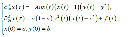(1)

where 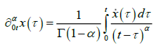and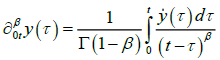 are the derivatives of fractional orders 0<α, β<1 in terms of Gerasimov-Caputo; Γ (x) is the Euler gamma function; x (t) is the effectiveness of new technologies; y (t) is the effectiveness of the return on assets; χ^* and y^* are the equilibrium steady-state solution of the system (1); n is the rate of accumulation; λ is the coefficient, determined out of the time series statistics; f(t) is the the external influence on the economic system; t ∈[0, T] the time coordinate, T is the time of process modeling; a and b are the initial conditions, given constants.

It should be noted that a non-linear system (1) if the values of the parameters are α=β=1 and f(t)=0 goes into Dubrovskiy model [4]. Therefore, it is obvious that the solution of a system (1) summarizes the solution of the Dubovskiy model. The solution of the nonlinear system (1) will be sought with the help of numerical methods – the theory of finite difference schemes. The time period [0, T] is divided into N equal parts with the increment τ. The approximation of the fractional derivatives in the equation (1) is performed according to the paper [18]. Then the system (1) can be written in the finite difference formulation in the form of:

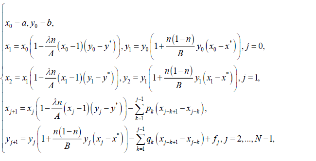(2)

Here

The solution (2) when α=β=1 and f_j=0 goes into the solution of the Dubrovskiy model [4]. Let us study the solution (2) depending on the different values of the fractional parameters and construct the phase paths. In this paper, the authors do not focus on the issues of stability or convergence of an explicit finite difference scheme (2).

The Results of Modeling and Their Discussion

The parameters of modeling were taken from the work written by Dubovskiy [4]: x^*=1.3, y^*=0.5, n=0.2, λ=2.25, x(0)=1.35, y(0)=0.5, T=250, α=β=1 (Figure 1).

Figure 1: The calculated curve a and the phase path b if f(t)=0.

Figure 1 shows the case, corresponding to the case of modeling of the Kondratiev cycle with the period of 50.1 years, described in the paper [5]. It can also be observed that the phase path (Figure 1b) has an ellipsoid closed shape, the equilibrium state of the system is called the center (Figure 2). The amplitude of oscillation is constant in this case (Figure 1a).

Figure 2: The calculated curve a and the phase path b if f(t)=δcos(ωt).

Figure 2 shows the case when the system (1) is influenced by the external periodic action f(t)=δcos(ωt). the investment cycles. The parameter values are δ=0.01 and ω=1. It can be concluded that the external periodic cycle gives a cycle with a period of about 7 years, which corresponds to a basic investment Juglar cycles [6], and the main cycle is equal to 60 years, which corresponds to the upper boundary of the Kondratiev cycle [2].

This combined model describes most flexibly the economic crises.

Figure 3 shows a case when f(t)=0, α=0.8 and β=1, and the other parameters remain unchanged.

Figure 3: The calculated curve a and the phase path b if α=0.8, β=1 and f(t)=0.

Figure 3a shows that the oscillation process is fading, and the phase path Figure 3b is not closed, the position of equilibrium of the system is called a stable focus. In this case, the cycles do not exist; however, if we introduce the function of the external action f(t)=δcos(ωt) which can be interpreted as the investment cycles, we come to the following result (Figure 4).

Figure 4: The calculated curve a and the phase path b if α=0.8, β=0.6 and f(t)=δcos(ωt), δ=0.5, ω=2.

Figure 3a shows that firstly the oscillation amplitude increases, and then enters the constant mode; it can be seen on the phase path in Figure 3b, which eventually enters the permanent regime or limit cycle, which can be used in the study of the Kondratiev cycles. The following figures (Figures 5 and 6) also show that the phase patches reach the limit cycles of various shapes.

Figure 5: The calculated curve a and the phase path b if α=0.8, β=0.8 and f(t)=δcos(ωt), δ=0.5, ω=2.

Figure 6: The calculated curve a and the phase path b if α=0.1, β=0.1 and f(t)=δcos(ωt), δ=0.5, ω=2.

Conclusions

The generalized Dubrovskiy model, which takes into account the memory effects (the economic barriers) in the economic system. The numerical solution of this model was obtained and the phase paths were built. It was shown that the introduction of the derivatives of fractional order results in the decaying processes; however, if there is any external periodic action in the system, the system enters the limit cycle, which can be considered whatever the economic cycle.

Further development of the mathematical model of the hereditary dynamic system (1) is the accounting of the dependence of the fractional indices α and β on time t [19]. This provides a more flexible model for the forecasting of the economic cycles.

Another line of study of the mathematical model (1) is a classification of its rest points, depending on the value of the fractional indices α and β to describe the different oscillation modes [20]. The fractional parameters α and β can be estimated using the experimental data of the economic indicators, for example, following the methods of the paper [21].

References

1. Parovik RI (2013) Modeling of the Selection of the Optimal Solution by the Administration of a Higher Education Institution, Agreed with the Management Decisions of Its Branches. Bulletin of KRAUNTS Physical and mathematical sciences 1: 5-11.
2. Kondrat'ev ND, Oparin DN (1928) Big Cycles of Conjuncture. Institute of Economics, Moscow.
3. Mensch G (1979) Stalemate in Technology .Innovations Overcome the Depression. Ballinger Pub Co, Cambridge.
4. Dubovskiy SV (1995) Object of Modeling – Kondratiev Cycle. Math modeling 7: 65-74.
5. Dubovskiy SV (2012) Modeling of the Kondratiev Cycles and Forecasting of the Crises. In: Akayev AA (ed.) Kondratiev Waves. The Aspects and the Prospects. Uchitel, Volgograd. pp. 179-188.
6. Dubovskiy SV (1993) Disaster Prediction (on the Example of the Cycles of N.D. Kondratiev). Social Sciences and Modernity 5: 82-91.
7. Makarov DV (2014) Economic and Mathematical Modeling of the Innovative Systems. Bulletin of KRAUNTS Physical and mathematical sciences 1: 66-70.
8. Makarov DV, Parovik RI (2016) A Generalized Mathematical Dubovskiy Model for Prediction of the Economic Crises. Scientific and Technical Gazette Volga 1: 74-77.
9. Nakhushev AM (2003) Fractional Calculus and Its Application. Fizmatlit, Moscow.
10. Boleantu M (2008) Fractional Dynamical Systems and Applications in Economy. Differential Geometry – Dynamical Systems 10: 62-70.
11. Yiding Y, Lei H, Guanchun L (2013) Modeling and Application of New Nonlinear Fractional Financial Model. Journal of Applied Mathematics.
12. Tejado I, Duarte V, Nuno V (2014) Fractional Calculus in Economic Growth Modeling. The Portuguese Case. In 2014 International Conference on Fractional Differentiation and its Applications (FDA'14).
13. Mendes RV (2008) A fractional Calculus Interpretation of the Fractional Volatility Model. Nonlinear Dyn 55: 395-399.
14. Zhenhua H, Xiaokang T (2015) A New Discrete Economic Model Involving Generalized Fractal Derivative. Advances in Difference Equations 65.
15. Shpilko YE, Solomko AA, Parovik RI (2012) Parameterization of the Samuelson Equation in the Evans Model on the Establishment of the Equilibrium Prices on the Market for One Product. Bulletin of KRAUNTS Physical and mathematical sciences 2: 33-36.
16. Samuta VV, Strelova VA, Parovik RI (2012) Nonlocal Model of the Solou Neoclassical Economic Growth. Bulletin of KRAUNTS Physical and mathematical sciences 2: 37-41.
17. Nakhusheva ZA (2012) On One One-Sector Macroeconomic Model of Long-Term Forecasting. Reports AMAN 14: 124-127.
18. Parovik RI (2015) Mathematical Modeling of the Linear Hereditarity Oscillators. KamGU named after Vitus Bering, Petropavlovsk-Kamchatsky.
19. Val´erio D, Costa JS da (2011) Variable-Order Fractional Derivatives and Their Numerical Approximations. Symposium on Fractional Signals and Systems 1: 470-483.
20. Petras I (2011) Fractional-Order Nonlinear Systems: Modeling. Analysis and Simulation. Springer, New York.
21. Bondarenko AN, Ivaschenko DS (2004) Numerical Algorithms of Solving of the Inverse Problems of Anomalous Diffusion . Collection of scientific papers NGTU 4: 59-64.