ISSN: 1204-5357
ISSN: 1204-5357
Edvard Evgenevich Nikulin*
Bauman Moscow State Technical University, Moscow, Russia
Denis Grigorevich Perepelitsa
Plekhanov Russian University of Economics, Russia
Olga Aleksandrovna zhdanova
Plekhanov Russian University of Economics, Russia
Sergey Alekseevich Smetanin
National Research University Higher School of Economics, Moscow, Russia
Elena Vladimirovna Nazarova
Plekhanov Russian University of Economics, Russia
Visit for more related articles at Journal of Internet Banking and Commerce
In this paper, we propose two fuzzy portfolio optimization models based on the Markowitz mean-variance approach. Uncertainty is an inherent property of the securities market, there turns of different types of securities can rarely be described statistically. Dealing with uncertainty, portfolio optimization theory began to move toward application of fuzzy mathematic. Besides presenting fuzzy models, this paper reveals the problem of reliability of the fuzzy model results. Solving this problem depends on the investor’s attitude to the model results. The first model involves fuzzy numbers to extend statistical data, the model returns the portfolio expected return and variance as fuzzy numbers. In addition to the problem formulated in the first model, the second model works on improvement of the indicators reliability. Finally, we provide a numerical example to illustrate the work of the proposed methods, as well as to compare the methods with each other and with the classical mean-variance method.
Portfolio Optimization, Fuzzy Optimization, Markowitz Model, Mean-Variance Model, Estimation of Results
Optimization of investment portfolio is one of the common financial problems which arise in the financial practice. Its solution allows investors finding the most effective way of investing capital in several types of securities. The main principles of the investment portfolio formation are reliability and return on investments, their stable growth and high liquidity. The purpose of the securities portfolio optimization is to create a securities portfolio that is consistent with the requirements of investor, and this is achieved by the distribution of securities in the portfolio.
Markowitz [1,2] introduced a mean-variance (MV) model which became a classical approach in the investment portfolio theory. Markowitz [1,2] assumed that the values of the securities’ returns were random variables distributed according to the normal law. Markowitz [1,2] believed that the investor, creating a portfolio, estimated only two indicators: the expected return and the standard deviation as a risk measure. Therefore, the investor must assess the profitability and standard deviation for each portfolio and choose the best portfolio in terms of the maximum return and the acceptable risk value.
The main problem is that the real processes taking place in the stock market are often unstable. Uncertainty is an inalienable property of the securities market, and the returns of different types of securities can rarely be described statistically. Thus, while dealing with uncertainty, the interest of scientists in portfolio optimization problems began to move toward applying the fuzzy mathematics proposed by Zadeh [3-5] which included an alternative approach to dealing with sets and probabilistic events.
The studies in the area of fuzzy portfolio optimization may be subdivided into three lines of research: fuzzy decision making models, models with fuzzy constraints or goals, and models with fuzzy numbers or possibility theory. The approaches to constructing the optimization models based on fuzzy decision making and fuzzy constraint/goals are investor-oriented. The models of this type engage fuzziness to describe vagueness in the investor’s desires.
Fuzzy Decision Making Models
Ramaswamy [6] considered a problem of forming a structured portfolio under uncertainty using the fuzzy decision theory framework; Ramaswamy [6] defined the decision maker’s degree of satisfaction by a membership function. Fang et al. [7] presented a model which employs fuzzification of risk, liquidity, expected return and fuzzy decision theory in order to form a portfolio in accordance with the investor’s degree of satisfaction.
Models with Fuzzy Constraints or Goals
Guo et al. [8] designed a fuzzy optimization model which takes into consideration the investor’s appetite. Parra et al. [9] have tried to define goals and constraints in a fuzzy form; the return, risk and liquidity were also presented as fuzzy numbers.
Models with Fuzzy Numbers or Possibility Theory [10,11]
AlmarazLuengo [12] and Lin et al. [13] described extensions of the Markowitz [1,2] optimization model using fuzzy values of the profit and risk. Hasuike et al. [14,15] proposed portfolio optimization models based on the scenarios approach with consideration of stochastic and fuzzy programming problems. The works of Tanaka et al. [16,17] present an optimization model for obtaining the upper and the lower possibility distributions which reflects the experts’ viewpoints. They expressed the optimization task as a quadratic programming problem which may be solved by standard optimization methods. Carlson et al. [18] modeled the security’s rate of return using the possibility distributions and proposed an algorithm for finding the exact optimal solution.
The goals of this paper are related to applications. We propose optimization models based on MV model with trapezoidal fuzzy numbers, as well as the estimation of the model results. In Section 2, we briefly provide necessary definitions from the fuzzy mathematics. In Section 3, we describe the design of the models. In Section 4, a numerical example is given to illustrate the work of the proposed models using different optimization algorithms and to compare the models with the classical MV model.
Preliminaries
In this section, we provide some necessary fuzzy mathematics definitions used in this work.
General Definitions
Definition 1: (fuzzy set) Let X be a nonempty set. A fuzzy set A in X is characterized by its membership function:
μA: X → [0, 1] (1)
μA(x) is interpreted as the degree of membership of element x in the fuzzy set A for each x ∈ X.
Definition 2: (support) Let A be a fuzzy subset of X; the support of A, denoted by sup (A), is the crisp subset of X whose elements all have nonzero membership grades in A.
 (2)
(2)
Definition 3: (normal fuzzy set) A fuzzy subset A of a classical set X is called normal if there exists an x ∈ X such that μA(x) =1. Otherwise, A is subnormal.
Definition 4: (γ-cut) Aγ-level set of a fuzzy set A of X is a non-fuzzy set denoted by [A]γ and is defined by:
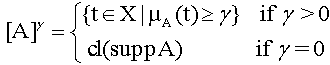 (3)
(3)
Where cl (suppA) denotes the closure of the support of A.
Definition 5: (convex fuzzy set) A fuzzy set A of X is called convex if [A]γ is a convex subset of X, ∀γ ∈[0,1]
Definition 6: (fuzzy number) A fuzzy number A is a fuzzy set of the real line with a normal, (fuzzy) convex and continuous membership function with bounded support.
Definition 7: (triangular fuzzy number) A fuzzy set A is called a triangular fuzzy number with the peak (or center) a, left width α>0 and right width β>0 if its membership function has the following form:
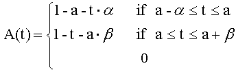 (4)
(4)
A =(a,α,β)
A triangle fuzzy number A is presented in Figure 1.

Figure 1: Triangle fuzzy number.
It can be verified that

A triangular fuzzy number with the center may be seen as a fuzzy quantity “x approximately equal to a” [2].
In the sequel, we will use the following form of the fuzzy number representation
A = (ax,bx,cx),(5)
Where
ax= a-α ,
bx= a,
cx = a+β.
This form makes the reduction of fuzzy arithmetic to the operations on intervals easer.
Definition 8: (trapezoidal fuzzy number) A fuzzy set A is called a trapezoidal fuzzy number with the tolerance interval [a,b], left width α>0 and right width β>0 if its membership function has the following form:
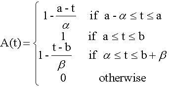 (6)
(6)
A = (a,b,α,β)
A trapezoidal fuzzy number A is presented in Figure 2.

Figure 2: Trapezoidal fuzzy number.
It can be shown that

We will use the representation:
A = (ax,bx,cx,dx), (7)
Where
ax = a - α,
bx= a,
cx= b,
dx = b + β.
Definitions of the Operations on Trapezoidal Fuzzy Numbers
We operate on fuzzy numbers using the intervals approach [19].
Let A1 and A2 be trapezoidal fuzzy numbers presented as
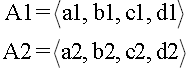
The four arithmetic operations are defined as follows:
• Addition
 (8)
(8)
• Subtraction
 (9)
(9)
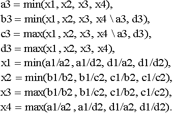
• Multiplication
 (10)
(10)
Where
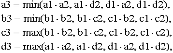
• Division
 (11)
(11)
Where
Expected Value and Variance of a Fuzzy Number
Let A be a trapezoidal fuzzy number such that
A = (a,b,α,β)
Expected Value
The expected value [18] of A is defined as
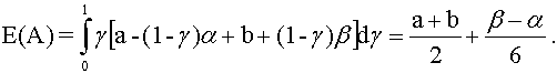 (12)
(12)
However, as we have already mentioned, we will represent the fuzzy number in the form of (7): A = (ax,bx,cx,dx)
Considering that
ax= a - α,
bx= a,
cx= b,
dx= b + β,
The expected value of A is transformed into the following expression:
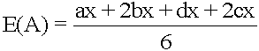 . (13)
Variance
The variance [20] of A is defined as
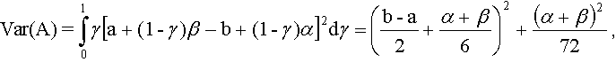 (14)
(14)
For A =(ax,bx,cx,dx) we will get
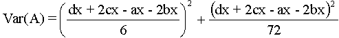 (15)
(15)
MV Model
The model we propose is based on the MV optimization approach. Hence, before starting the description of the proposed model, we have to consider the main principles of optimization by Markowitz [1,2].
In his theoretical studies, Markowitz [1,2] assumed that the values of the securities returns are random variables distributed according to the normal law. Markowitz [1,2] believed that the investor, creating the portfolio, estimates only two indicators: the expected value and standard deviation (these two indicators determine the probability density of the random number with the normal distribution). Therefore, the investor must estimate the expected value and standard deviation values for each portfolio and choose the best portfolio that satisfies his/her desires for maximum return with an acceptable risk value.
This approach presumes that, at a given moment of time, the investor has a specific amount of money to invest. This money will be invested for a certain period of time called the period of ownership. At the end of the period of ownership, the investor sells the securities that were purchased at the beginning of the period, and then either use the resulting income on consumption, or reinvest it in various securities.
In general, MV optimization model involves the following assumptions
• The expected value is taken as the security return;
• The standard deviation is regarded as the security risk;
• The historical data used in the calculation of profitability and risk fully reflect the future values;
• The relationships between securities are expressed by the correlation coefficients.
Markowitz [1,2] claimed that the maximum revenue from the portfolio should not be the basis for decision-making because of the risk elements. To minimize the risk, we need to diversify the portfolio. Reducing the risk, however, means reducing profitability. In fact, we need a portfolio in which the levels of risk and income would be acceptable for the investor.
MV optimization problem may be described as follows [4]:
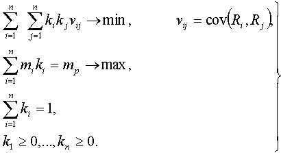 (16)
(16)
Where
mp is the value of the portfolio return,
ki is the share of securities in the portfolio,
mi is the expected value of the i -th security return Ri : mi= MRi,i =1,...n,.
Fuzzy Optimization Model
Having considered the basics of the classical MV optimization, we are going to present an optimization model which is an extension of MV model. It provides possibility results in the form of fuzzy numbers and the estimation of these results. The investor may choose the optimization of the expected return and risk only, then the estimation serves as an indicator of the obtained data reliability; alternatively, choosing optimization of the expected return, risk and estimation parameters, the investor gains the possibility to improve the result reliability.
To introduce fuzziness into MV model, we start with the observation that during the trading day the value of the security changes continuously, starting with opening price, reaching a minimum and a maximum, and finishing with closing price. We define security’s return as a trapezoidal fuzzy number.
Suppose that the i-th security in every trading day may be characterized by four parameters: the opening price Sitopen, the closing price Sitclose,the high Sithighand the low Sitlowprices, where i = 1, 2, … N is the number of the considered type of securities, t = 1, 2 … T is the number of the trading day.
Then the maximum return of the security is the ratio of the maximum possible profit for the selected period to the minimum possible cost of its purchase:
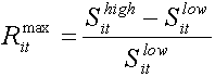 (17)
(17)
The minimum return of the security is:
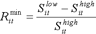 (18)
(18)
The average return values of the security are:
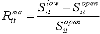 (19)
(19)
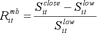 (20)
(20)
The definitions of Ritma and Ritmb are based on the fact that there is 100% possibility to sell shares at the low price if they were purchased at the opening price and to sell shares at the closing price if they were purchased at the low one [20].
Now the yield of the security can be presented in a trapezoidal fuzzy form:
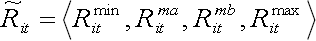 (21)
(21)
The expected return of the security is as follows:
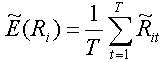 (22)
(22)
Then the coefficients of covariance matrix for the yields of securities are defined as:
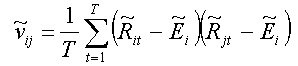 (23)
(23)
The expected return of the portfolio is a trapezoidal fuzzy number, because it is formed by the expected returns of the securities, which are trapezoidal fuzzy numbers:
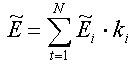 (24)
(24)
The variance of the portfolio is defined similarly to its definition in the Markowitz model, but it is now a trapezoidal fuzzy number:
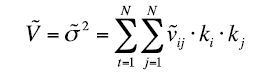 (25)
(25)
Next we can define the function of portfolio effectiveness which we are to optimize:
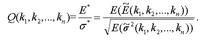 (26)
(26)
An optimization problem can be represented in the following form:
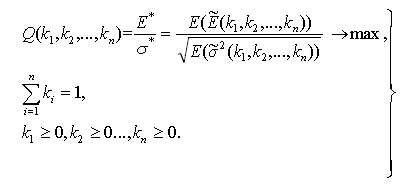 (27)
(27)
Where  and
and  are expected values of the fuzzy numbers that characterize the values of the portfolio expected return and variance.
In addition, we propose an optimization problem which includes minimization of the fuzzy numbers of variances, thus making them more ‘crispy’ and more precise with consideration of their fuzzy range. The variances of the fuzzy numbers serve as indicators of reliability of the model results.
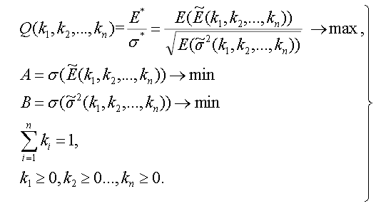 (28)
(28)
To solve the first optimization problem (27), we employ the genetic (GA) [21], pattern search (PS) and interior point (IP) algorithms [22].
To solve the second optimization problem (28), we use the minimax (MM) and GA methods.
In solving the optimization problem for the portfolio given in Section 4, the deterministic methods provide better results in terms of accuracy and performance time than GA, but with the increasing dimensions, the situation may change in favor of GA. In any case, we recommend using several different algorithms for solving the optimization problem. Using the deterministic methods after having performed the optimization by heuristic methods can also give advantage.
In order to demonstrate the results of the proposed model, a numerical example is presented in this chapter (Table 1). We chose a portfolio which includes shares of seven companies (Barrick Gold Corporation; Alere, Inc.; Shell Midstream Partners, L.P.; Tesla Motors, Inc.; International Business Machines Corporation; Alphabet Inc.; MasterCard Inc.) from Nasdaq stock market with the time frame from 16.06.16 to 16.07.16.
Table 1: Results of MV portfolio optimization.
| k1 | k2 | k3 | k4 | k5 | k6 | k7 | E, *1e-3 | σ, *1e-3 | Q | |
|---|---|---|---|---|---|---|---|---|---|---|
| GA | 0.112 | 0.116 | 0.136 | 0.174 | 0.102 | 0.127 | 0.233 | 0.659 | 6.835 | 0.096 |
| PS | 0 | 0.097 | 0 | 0.594 | 0 | 0.029 | 0.280 | 1.401 | 8.364 | 0.168 |
| IP | 0.008 | 0.091 | 0.006 | 0.513 | 0.007 | 0.029 | 0.346 | 1.418 | 8.552 | 0.166 |
MV optimization (16) was used to estimate the expediency of proposed model.
The results of solving the first fuzzy optimization problem (27) are presented in Table 2. We may see that the solutions of the first optimization problem are better than the results of MV optimization; this is explained by the fact that fuzzy variables are extension of crisp variables. We obtain extensions of the risk and expected return functions, hence the range of the optimized function increases.
Table 2: Results of the first fuzzy portfolio optimization problem.
| K1 | k2 | k3 | k4 | k5 | k6 | k7 | E*, *1e-3 | σ*, *1e-3 | Q | A | B | |
|---|---|---|---|---|---|---|---|---|---|---|---|---|
| GA | 0.045 | 0.062 | 0.068 | 0.341 | 0.123 | 0.063 | 0.298 | 0.783 | 4.025 | 0.207 | 0.071 | 0.006 |
| PS | 0.001 | 0.091 | 0 | 0.549 | 0 | 0.034 | 0.325 | 1.009 | 4.386 | 0.256 | 0.069 | 0.005 |
| IP | 0 | 0.075 | 0 | 0.533 | 0 | 0.008 | 0.384 | 1.098 | 4.777 | 0.258 | 0.070 | 0.005 |
A and B in the Table 1 are variances of fuzzy numbers; the smaller these indicators are, the more reliable are the values of E*, σ* and Q.
The results from solving the second fuzzy optimization problem (28) are presented in Table 3; in this case, the optimization includes the minimization of A and B.
Table 3: Results of second fuzzy portfolio optimization problem.
| k1 | k2 | k3 | k4 | k5 | k6 | k7 | E*, *1e-3 | σ*, *1e-3 | Q | A | B | |
|---|---|---|---|---|---|---|---|---|---|---|---|---|
| MM | 0 | 0 | 0.365 | 0.465 | 0.170 | 0 | 0 | 0.309 | 5.012 | 0.062 | 0.049 | 0.003 |
| GA | 0.001 | 0.005 | 0.010 | 0.832 | 0.127 | 0.003 | 0.022 | 0.786 | 6.189 | 0.127 | 0.050 | 0.003 |
The value of portfolio effectiveness function is lower, which can be explained by the desire to maximize the results reliability. We may see that the values of A and B are significantly lower than in the first fuzzy optimization problem. It reveals the problem of investor’s attitude to the reliability of the model results. Thus, the model allows additionally taking into account the investor’s concern for the results reliability.
In this paper, we have considered fuzzy models of portfolio optimization based on the MV optimization approach: the first model involves fuzziness of securities prices, which takes place in the conditions of real stock market processes. The second model deals with fuzzy optimization of portfolio effectiveness function similarly to the first model, but it also includes a method of estimating the results reliability. The proposed models have been tested on the trial investment portfolio. The testing of the models has showed their aptitude and revealed the problem of investor’s attitude to the data reliability proposed by the model. The results of solving the first fuzzy optimization problem are better than the results of MV optimization in terms of risk and expected return; it can be explained by the fact that fuzzy variables are extension of crisp variables. Using fuzzy numbers for defining portfolio parameters enables us to work with an extended range of the portfolio effectiveness function. The results of solving the second fuzzy optimization problem are better than results of the first problem in terms of reliability, but worse in terms of risk and expected return, which is quite obvious: the safer data we want to get, the smaller our expected return and risk are going to be.
In the continuation of this work, we would like to investigate a problem of investor’s level of data confidence and on this basis provide a model which would consider it.
The code of the model is written in the MATLAB. One can download it from http://www.mathworks.com/matlabcentral/fileexchange/58886-fuzzy-portfoliooptimization
Copyright © 2026 Research and Reviews, All Rights Reserved