Credit Risk Assessment Using Survival Analysis For Progressive Right-Censored Data: A Case Study in Jordan

Jamil J Jaber^*

Department of Risk Management and Insurance, Faculty of Management and finance, University of Jordan, Jordan

Noriszura Ismail

School of Mathematical Sciences, Faculty of Science and Technology Universiti Kebangsaan Malaysia, Malaysia

Siti Norafidah Mohd Ramli

School of Mathematical Sciences, Faculty of Science and Technology Universiti Kebangsaan Malaysia, Malaysia

*Corresponding Author:

Jamil J Jaber
Department of Risk Management and Insurance
Faculty of Management and finance
University of Jordan, Jordan
Tel: +962 6 535 5000
E-mail: j.jaber@ju.edu.jo, jameljaber2011@hotmail.com

Visit for more related articles at Journal of Internet Banking and Commerce

Abstract

In credit risk management, the Basel Committee provides a choice of three approaches for financial institutions to calculate the required capital; standardized approach, Internal Ratings-Based (IRB) approach, and Advanced IRB approach. The IRB approach is usually preferred compared to the standard approach due to its higher accuracy and lower capital charges. The objective of this study is to use several parametric models (exponential, log-normal, gamma, Weibull, log-logistic, Gompertz) and non-parametric models (Kaplan-Meier, Nelson-Aalen) to estimate the probability of default which can be used for evaluating the performance of a sample of credit risk portfolio. The models are fitted to a sample data of credit portfolio obtained from a bank in Jordan for the period of January 2010 until December 2014. The best parametric and non-parametric models are selected using several goodness-of-fit criteria, namely MSE, AIC and BIC for parametric models and SE and MAD for non-parametric models. The estimated default probability is then applied to forecast the credit risk of a corporate portfolio at 99.9% confidence level and several time horizons (3 months, 6 months, 9 months, 1 year). The results show that the Gompertz distribution is the best parametric model, whereas the Nelson-Aalen estimator is the best non-parametric model for predicting the probability of default of the credit portfolio.

Keywords

Survival; Credit Risk; Time to Default

Introduction

The assessment of credit risk is crucial for financial institutions such as banks and insurance companies. The Basel II Capital Structure published by the Basel Committee supervision in June 2006 requires that the financial institutions hold a minimum capital to cover the exposures of market, credit, and operational risks. Therefore, all banks and financial institutions are required to assess their portfolio risks, including credit risk.

The Basel Committee provides a choice of three approaches for calculating the required capital: standardized approach (low complexity, low accuracy and high capital charge), Internal Ratings-Based approach (IRB) (medium complexity, medium accuracy, and medium capital charge), and advanced IRB approach (high complexity, high accuracy and low capital charge). The standardized approach provides improved risk sensitivity compared to the Basel I requirement. The two IRB approaches, which rely on the bank’s internal risks rating, are considerably more sensitive to risks.

Based on the literature, several methodologies for modeling credit risk have been proposed since the introduction of the classical Z-score model by Altman [1] which is applied to verify the grant of credit of an applicant. As examples, the ZETA discriminant analysis model, which is constructed through the linear function of market variables and accounting, is able to differentiate between reimbursement and non-reimbursement of a credit borrower. The logistic regression model, which assumes that the cumulative probability has a logistic functional form, is able to predict the probability of a borrower’s default. Recently, the artificial neural network (ANN), which uses the artificial intelligence (AI) approach, has been considered for credit scoring [2-5].

The modelling of credit risk based on survival analysis was first introduced by Narain [6] who applied the survival model to a 24-months credit data. Later, Thomas et al. [7] used the accelerated life exponential model to a sample data of 24-months credit information and compared the model with Weibull, Cox non-parametric and logistic regression models. Their study showed that the use of survival analysis in credit scoring is superior to the conventional strategies due to the support of estimated survival times in making credit decision. Another example can be found in Cao et al. [8] who studied several consumer credit risk models via survival analysis by fitting parametric models (Pareto, F-distribution, normal distribution, Weibull distribution and Cauchy distribution), nonparametric model (Kaplan-Meier), and semi-parametric model (Cox) to the right censored data. Several other parametric, semi-parametric and non-parametric models were also applied to credit portfolio data, and these techniques can be found in Stepanova et al. [9], Malik et al. [10] and Man [11]. Recently, Luo et al. [12] applied a regression spline based on a discrete time survival model, and compared the model’s performance with the classical Cox model. In summary, a common feature of all these studies is that the survival analysis with parametric, semi-parametric and nonparametric techniques have been applied for modeling the probability of default of credit portfolios.

The objective of this paper is to estimate the probability of default (PD) using parametric and non-parametric models. The parametric and non-parametric models are fitted to the right-censored data obtained from a bank in Jordan for the period of January 2010 until December 2014. The estimated PD is then used for predicting the performance of credit risk of a corporate portfolio. The rest of the paper proceeds as follows. Section 2 provides the methodology, while section 3 provides the data description and results. Finally, section 4 provides the conclusions.

Methodology

Worst-Case Default Rate (WCDR)

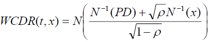
The capital requirements for credit risk in Basel II Internal Rating Based (IRB) can be formulated using the Risk-Weighted Assets (RWA) formula. One of the elements required in the RWA formula is the Worst-Case Default Rate (WCDR) that depends on Vasicek’s Gaussian copula model. The WCDR equation is:

   (1)

Where WCDR is the worst–case default rate for a time horizon t (usually one year), x is the confidence level (which is defined at 99.9% by Basel II regulators), PD is the probability that a loan will default at time t, and ρ is the copula correlation parameter for each pair of loans.

Based on empirical research, the Basel II assumes that the copula correlation parameter, ρ , and the PD has the following relationship: .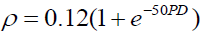

As an example, suppose that a bank has a total of USD50 million of exposures, a oneyear PD of 1.5% for each loan, the loss of 45% given the default of each loan, and the estimated correlation copula parameter of

Therefore, the WCDR(1,0.999) is 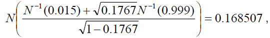indicating that the 99.9% worst case default rate is 16.85%, and the losses when this worst case occurs amounted to USD3.79 million (USD50 mil  0.1685  0.45). This USD3.79 million is also the estimate of value-at-risk (VaR) for the credit portfolio at a one-year time horizon and 99.9% confidence level.

The focus of this study is the estimation of PD of a credit portfolio based on several parametric and non-parametric models. The best model for PD is then selected using several goodness-of-fit tests. The estimated PD is then applied to forecast the WCDR at confidence level 99.9% and several time horizons (t=3 months, 6 months, 9 months, 1 year).

Survival Model

Survival analysis is a statistical method whose outcome variable of interest is the time to the occurrence of an event which is often referred to as failure time, survival time, or event time. Survival data can be divided into three categories; complete, censored and truncated. Complete data is the ideal data that contains the begin and end dates of which the event time is determined. Censored and truncated data are also called missing data due to the unavailability of information on the begin or end dates.

An observation is said to be truncated from below (above) or left (right) truncated, if when it is at or below (above) the truncation point it is not recorded, but when it is above (below) the truncation point it is recorded at its observed value. On the other hand, an observation is said to be censored from above (below) or right (left) censored, if when it is at or above (below) the censored point it is recorded as being equal to the censored point, but when it is below (above) the censored point it is recorded at its observed value [13].

Right censored data can be divided into three types: type I, type II and type III. Type I and type II are also called the singly censored data, while type III is also called the progressively censored data [14]. Another commonly used name for the type III censoring is random censoring.

Besides right censoring, there are also cases of left censoring and interval censoring. Left censoring occurs when it is known that the event occurred prior to time a, but the exact time of occurrence is unknown. On the other hand, interval censoring occurs when the event of interest is known to have occurred between times a to b.

Our study uses the progressive right censored data for estimating the PD of a sample of credit portfolio in Jordan. The three main reasons for using the progressive censoring are: the period of study is fixed, the borrowers can enter the study at different times during the fixed period, and the borrowers may or may not default before the end of study.

Suppose that T is the length of time before default. The randomness of T can be described in four standard ways; density function, survival function, distribution function and hazard function.

The probability that the failure time occurs at exactly time t is given by the density function:

   (2)

The probability that the time to event (T) is larger than a fixed time t is given by the survival function:

   (3)

The probability that the time to event (T) is smaller or equal than a fixed time t is the distribution function:

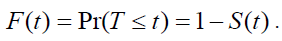   (4)

Finally, the incidence rate, or the instantaneous risk or force of mortality, or the event rate at time t among those at risks at time t, is known as the hazard rate function:

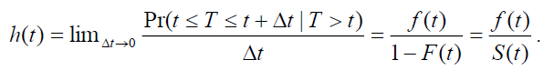   (5)

Therefore, the cumulative hazard rate function can be calculated as:

   (6)

Parametric Models

Fitting a parametric distribution to a sample of censored data has several advantages. Firstly, the survival and density functions for a parametric model, S(t) and f(t), are fully specified, and thus, can be easily used to estimate the quintiles of different distributions. In addition, the statistical tests involving the testing of parameters are more powerful and efficient. In short, the parametric distributions provide more statistical inference than the non-parametric distributions. Examples of commonly used parametric distributions for estimating survival curves are the exponential, log-normal, gamma, Weibull (proportional hazards), log-logistic and Gompertz. Table 1 provides the density, survival, hazard, and cumulative hazard functions for the commonly used parametric models.

Table 1: Common parametric models for estimating survival curves.

Model	Parameters	Probability density function f (x)	Survival function S(x)	Hazard function h(x)	Cumulative hazard function H(x)
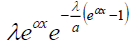
Exponential	rate (λ)			λ
Log-normal	mean (μ) s.d. (σ)
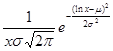Gamma	shape (α) rate (β)
Weibull (proportional hazards)	shape (α) rate (β)
Log-logistic	shape (α) scale (β)
Gompertz	shape (α) rate (β)
**Φ is the cumulative distribution function of standard normal distribution

Let t_i, i=1,2,….,n, be the sample of event times for loan. Let c_i=1 if t_i is an observed default time, and c_i=0 if the observation is a censored loan data. Most commonly, t_i is a right-censored data (c_i=0), meaning that the observed data is a non-default case and has to exit the study due to the end of observation period.

The likelihood for the parametric model is

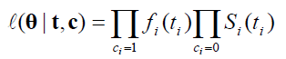   (7)

where the density fi(ti) is the likelihood of an observed default time and Si(ti) is the likelihood of a censored data. The estimated parameters can be obtained by maximizing the likelihood in eqn (7).

Non-Parametric Models

The non-parametric or distribution-free technique is less effective than the parametric method when the survival time is known to follow a theoretical distribution. However, the non-parametric model is more proficient when the appropriate theoretical distribution is not known.

In the case of censored data, two common non-parametric techniques can be applied: Kaplan-Meier (KM) which is also known as product limit estimator (Kaplan and Meier) and Nelson-Aalen (NA) estimator (Aalen). The KM estimator estimates the median of survival function, whereas the NA estimator estimates the cumulative hazard rate function. The main advantage of using these two estimators is that they consider censored data.

Suppose m individuals experience defaults in a portfolio of loans. Let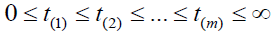 be the observed default times. In addition, let r_j be the number of loans at risk just before t_j, j = 1,2,...,m, and d_j be the number of observed defaults at t_j. The KM estimator of survival function S(t) is

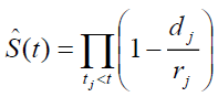   (8)

where dj is the number of observed defaults at time tj, and rj is the number of loans at risks in the portfolio at time tj. The unbiased KM estimator of the cumulative hazard rate is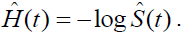

It should be noted that the KM estimator is a step function that does not change between default times, nor at the time of censoring. The estimator only changes at the time of each default.

The Nelson-Aalen (NA) estimator is used to estimate the cumulative hazard rate, Hˆ (t) , and is defined by

where d_j is the number of defaults at time t_j, and r_j is the number of loan at risks at time t_j. The NA estimator of the survival function can be obtained using .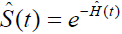

Model Selection

We use five types of accuracy criteria to select the best model; mean square error (MSE), standard error (SE), Bayesian information criterion (BIC), Akaike information criterion (AIC) and mean absolute deviation (MAD). The mean square error (MSE) is 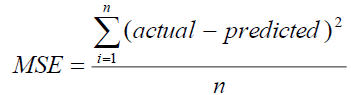where n is the sample size. The Bayesian information criterion (BIC) is based on the maximum likelihood estimates of the model parameters [15] which penalizes a sample with larger size and larger number of parameters, and the formula is BIC= - 2l + kp, where l is the log likelihood of the estimated model, p is the number of parameters, and k=log n. The Akaike information criterion (AIC) is also based on the maximum likelihood estimates of model parameters [16], but penalizes a sample with larger size. The formula AIC= - 2l + k*p, is where l is the log likelihood of the estimated model, p is the number of parameters, and k*=2. The standard error (SE) is usually estimated by the sample estimate of standard deviation of population (sample standard deviation) divided by the square root of sample size (assuming independence), 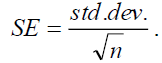Finally, the mean absolute deviation (MAD) is 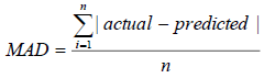where n is the sample size.

Results

Data Description

The sample data of credit portfolio obtained for this study are collected from a bank in Jordan and contain confidential information on credit of loans. The monthly data of the credit portfolio were collected from January 2010 until December 2014. The size of portfolio is 4393, while the total number of defaults throughout the 5-year period is 495. For the sample data, a borrower is declared default when his/her cash instalment is not paid within 3 months.

Table 2 provides the risk exposures (number of loans at risk) and number of defaults in each year. The highest number of defaults occurred in the second year, and the highest number of defaults per exposure also occurred in the same year (168 defaults from 1125 exposures). Table 3 provides the summary statistics for the monthly data. The average monthly exposure is 73, while the average number of defaults per month is 8.

Table 2: Number of exposures and defaults in each year.

Table 3: Summary statistics for credit data (monthly).

Parametric Model

The estimated parameters for the parametric models can be obtained by maximizing the likelihood shown in eqn (7). The R software with flexsurv package is used in this study to fit the parametric models via maximum likelihood estimation [17]. The best parametric model is then selected using several goodness-of-fit criteria such as MSE, AIC and BIC.

Table 4 provides the estimated parameters, together with the standard errors, lower bounds and upper bounds. The MSE, AIC and BIC are also provided, and the best model is chosen based on the smallest MSE, and the largest AIC and BIC. The results in Table 4 show that the Gompertz distribution is the best parametric model since it has the smallest MSE, and the largest AIC and BIC. The maximum likelihood estimate of the Gompertz parameters are α=0.0276 and λ=0.0196

Table 4: Estimated parameters and goodness-of-fit criteria for parametric models.

For further comparison, Figure 1 shows the curve of survival function for all of the fitted parametric models. The fitted curves are compared to the non-parametric curve from Kaplan-Meier estimation. The graphs illustrate that the survival curve of Gompertz model is closest to the non-parametric curve compared to other models.

Figure 1: Fitted survival function for parametric models. a) Exponential distribution, b) Log-Normal distribution, c) Gamma distribution, d) Weibull distribution, e) Log-logistic distribution, f) Gompertz distribution.

Non-Parametric Model

The R software with flexsurv package is used in this study to fit the non-parametric models to the sample data [17]. The package can be used to estimate the Kaplan- Meier’s (KM) survival function, Sˆ(t) , and the cumulative hazard function, Hˆ (t) . The estimation of Nelson-Aalen (NA) is carried out using the survival function, Sˆ(t) , via Cox regression model without covariates [18]. The cumulative hazard function, Hˆ (t) , is then estimated using 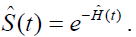The best non-parametric model is selected using several goodness-of-fit criteria such as SE and MAD.

Table 5 provides information on the exposure (number of risk) and number of defaults in each month for the sample data [19,20]. The Table 5 also provides the estimates of survival and cumulative hazard functions for the NA and KM in each month. The results indicate that the survival estimates of NA are slightly larger than KM over the 60 months period. On the contrary, the estimates of cumulative hazard of KM are larger than NA over the study period.

Table 5: Estimates of and for non-parametric models.

Time (in mth)	Monthly exposure	# of non-censoreds	Nelson-Aalen (NA)			Kaplan-Meier (KM)
					Std. err			Std. err
1	272	254	0.058	0.944	0.0034	0.060	0.942	0.0035
2	160	145	0.093	0.911	0.0043	0.095	0.909	0.0043
3	192	178	0.138	0.871	0.0050	0.141	0.868	0.0051
4	80	67	0.156	0.856	0.0053	0.159	0.853	0.0054
5	112	100	0.183	0.833	0.0056	0.187	0.830	0.0057
6	48	38	0.193	0.824	0.0057	0.198	0.821	0.0058
7	112	101	0.222	0.801	0.0060	0.227	0.797	0.0061
8	64	55	0.238	0.788	0.0062	0.243	0.784	0.0062
9	48	40	0.250	0.779	0.0063	0.255	0.775	0.0063
10	64	55	0.267	0.766	0.0064	0.272	0.762	0.0065
11	49	39	0.279	0.757	0.0065	0.284	0.753	0.0066
12	64	55	0.296	0.744	0.0066	0.301	0.740	0.0067
13	73	61	0.316	0.729	0.0067	0.321	0.726	0.0068
14	81	67	0.338	0.714	0.0069	0.343	0.710	0.0069
15	121	92	0.368	0.692	0.0070	0.374	0.688	0.0071
16	101	83	0.398	0.672	0.0071	0.404	0.668	0.0072
17	115	102	0.435	0.648	0.0073	0.442	0.643	0.0073
18	130	112	0.477	0.621	0.0074	0.485	0.616	0.0075
19	112	108	0.520	0.594	0.0075	0.529	0.589	0.0076
20	109	96	0.560	0.571	0.0076	0.570	0.566	0.0076
21	97	85	0.597	0.550	0.0076	0.608	0.545	0.0077
22	78	68	0.628	0.533	0.0077	0.639	0.528	0.0077
23	56	46	0.650	0.522	0.0077	0.661	0.516	0.0077
24	52	37	0.668	0.513	0.0077	0.680	0.507	0.0077
25	67	57	0.697	0.498	0.0077	0.709	0.492	0.0078
26	72	63	0.729	0.482	0.0077	0.742	0.476	0.0078
27	83	72	0.768	0.464	0.0077	0.781	0.458	0.0078
28	67	64	0.804	0.448	0.0077	0.818	0.442	0.0078
29	74	71	0.845	0.429	0.0077	0.860	0.423	0.0077
30	90	85	0.897	0.408	0.0077	0.913	0.401	0.0077
31	76	70	0.942	0.390	0.0076	0.959	0.383	0.0076
32	57	51	0.977	0.377	0.0076	0.995	0.370	0.0076
33	61	56	1.016	0.362	0.0075	1.035	0.355	0.0075
34	53	50	1.053	0.349	0.0075	1.072	0.342	0.0075
35	36	33	1.079	0.340	0.0075	1.098	0.334	0.0075
36	47	44	1.113	0.329	0.0074	1.133	0.322	0.0074
37	49	46	1.151	0.316	0.0073	1.172	0.310	0.0073
38	59	56	1.199	0.302	0.0073	1.221	0.295	0.0072
39	54	54	1.247	0.287	0.0072	1.271	0.281	0.0071
40	48	46	1.291	0.275	0.0071	1.315	0.268	0.0071
41	63	60	1.350	0.259	0.0070	1.376	0.253	0.0069
42	59	53	1.406	0.245	0.0069	1.434	0.238	0.0068
43	70	60	1.474	0.229	0.0067	1.504	0.222	0.0067
44	65	63	1.551	0.212	0.0066	1.584	0.205	0.0065
45	62	58	1.628	0.196	0.0064	1.664	0.189	0.0063
46	46	41	1.687	0.185	0.0063	1.725	0.178	0.0062
47	35	35	1.741	0.175	0.0061	1.781	0.168	0.0061
48	42	39	1.805	0.164	0.0060	1.847	0.158	0.0059
49	29	28	1.855	0.157	0.0059	1.898	0.150	0.0058
50	38	36	1.921	0.146	0.0058	1.967	0.140	0.0056
51	30	27	1.975	0.139	0.0056	2.022	0.132	0.0055
52	36	30	2.039	0.130	0.0055	2.088	0.124	0.0054
53	29	25	2.097	0.123	0.0054	2.147	0.117	0.0053
54	48	40	2.195	0.111	0.0052	2.251	0.105	0.0050
55	42	37	2.298	0.100	0.0050	2.360	0.094	0.0048
56	68	61	2.491	0.083	0.0046	2.575	0.076	0.0044
57	33	30	2.612	0.073	0.0044	2.704	0.067	0.0042
58	35	31	2.757	0.064	0.0041	2.859	0.057	0.0039
59	29	23	2.884	0.056	0.0039	2.996	0.050	0.0037
60	151	118	3.666	0.026	0.0026	4.517	0.011	0.0019

In terms of standard error of Sˆ(t) , the estimates of KM are larger than NA during the first 31 months, followed by almost no differences between both estimates over the next four months. After that, the estimates of NA are larger than KM in the duration of 36 to 60 months.

For a more consistent measure of goodness-of-fit, we use the total difference of 99% confidence interval (CI) and the MAD as our selection criteria for choosing the best non-parametric model [21-25]. The results of the selection criteria (99% CI difference and MAD) for the non-parametric models are provided in Table 6. The results show that the NA estimator is better than the KM estimator, as shown by the smaller values of 99% CI difference and MAD for the estimates of survival function, cumulative hazard function and standard error.

Table 6: Estimated parameters and goodness-of-fit criteria for parametric models.

For further comparison, Figure 2 shows the fitted curve of survival function for the KM and NA models. The plots show that both estimates are similar, and have decreasing patterns throughout the 5-year period.

Figure 2: Fitted survival function for non-parametric models. a) NA, b) KM, c) NA and KM.

Worst Case Default Rate for Credit Portfolio

As mentioned previously, the focus of this study is to estimate the probability of default (PD) which can be applied to forecast the worst case default rate (WCDR) of a credit portfolio at confidence level x and time horizon t. The WCDR can be estimated using Vasicek’s Gaussian copula model as shown in eqn (2), while the copula correlation parameter can be obtained using the empirical results of Basel II where 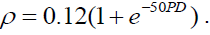Assuming that the PD follows the Gompertz model (best parametric model) with parameters α =0.0276 and λ =0.0196, the estimates of PD, copula correlation and WCDR at 99.9% confidence level and several time horizons are provided in Table 7.

Table 7: Default probability, copula correlation and WCDR.

The results in Table 7 show that both PD and WCDR increase during the one-year period, but the copula correlation decrease in the same period. As expected, the PD and WCDR has a positive relationship (higher PD resulted in higher WCDR), while the PD and copula correlation has a negative relationship (higher PD resulted in lower copula correlation) [26,27].

Conclusion

This paper has estimated the probability of default (PD) by fitting parametric and nonparametric models to a sample of credit portfolio obtained from a bank in Jordan for the period of January 2010 until December 2014 [28-31]. The best parametric model is the Gompertz model with parameters α =0.0276 and λ =0.0196, while the best nonparametric model is the Nelson-Aalen estimator.

The parametric distribution has the advantage of providing more statistical inferences compared to the non-parametric distribution. The survival and density functions of parametric distribution are fully specified and can be easily used to estimate different quintiles for different distributions. The parametric model also has more tests that are statistically powerful and efficient. However, the non-parametric model is more proficient than the parametric model when the appropriate theoretical distribution is not known. The main advantage of using the non-parametric models of KM and NA estimators is that both estimators consider censored data and the estimates of survival and cumulative hazard be computed using simple formulas.

In this study, the estimated PD from Gompertz model is used for forecasting the worst case default rate (WCDR) of a credit portfolio at 99.9% confidence level and several time horizons. The WCDR is one of the elements required to calculate the Risk- Weighted Assets (RWA), which is the formula for calculating the capital requirements in Basel II Internal Rating Based (IRB) [32-34]. The results show that the estimates of PD and WCDR increase during the one-year period, while the estimates of copula correlation decrease during the same period. The results are expected since the PD and WCDR has a positive relationship as shown by the WCDR formula in eqn (1), while the PD and copula correlation has a negative relationship as shown by the formula,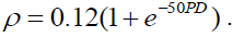

For further study, we plan to incorporate the macroeconomic effects in the prediction of PD. In addition, the concept of risk-transfer through insurance policies for reducing the credit risk of portfolio can be considered, and studies on the prediction of PD which takes into account insurance policies for reducing credit risks will be carried out in future studies.

References

1. Altman EI (1968) Financial ratios, discriminant analysis, and the prediction of corporate bankruptcy. Journal of Finance 23: 589-611.
2. Altman E, Saunders A (1998) Credit risk measurement: Developments over the last 20 years. Journal of Banking and Finance 21: 1721-1742.
3. Wang Y, Wang S, Lai KK (2005) A fuzzy support vector machine to evaluate credit risk, IEEE Transactions on Fuzzy Systems 13: 820-831.
4. Bellotti T, Crook J (2009) Support vector machines for credit scoring and discovery of significant features. Expert Systems with Applications 36: 3302-3308.
5. Alaraj M, Abbod M, Al-Hnaity B (2015) Evaluation of Consumer Credit in Jordanian Banks: A Credit Scoring Approach. 17th UKSIM-AMSS International Conference on Modelling and Simulation.
6. Narain B (1992) Survival analysis and the credit granting decision. In: Thomas L, Crook JN, Edelman DB (eds.) Credit Scoring and Credit Control. OUP: Oxford. pp: 109-121.
7. Thomas LC, Banasik J, Crook N (1999) Not if but when Loans Default. J Operations Research Society 50: 1185-1190.
8. Cao R, Vilar JM, Devia A (2009) Modelling consumer credit risk via survival analysis. SORT 33 (1) January-June 2009, 3-30.
9. Stepanova M, Thomas LC (2002) Survival analysis methods for personal loan data. Operations Research 50: 277-289. http://dx.doi.org/10.1287/opre.50.2.277.426
10. Malik M, Thomas L (2006) Modelling credit risk of portfolio of consumer loans, University of Southampton. School of Management Working Paper Series No. CORMSIS-07-12.
11. Man R (2014) Survival analysis in credit scoring: A framework for PD estimation. University of Twente.
12. Luo S, Kong X, Nie T (2016) Spline Based Survival Model for Credit Risk Modeling. European Journal of Operational Research.
13. Klugman SA, Panjer HH, Willmot GE (2012) Loss Models from Data to Decisions. 4th Edition. Wiley.
14. Cohen AC (1965) Maximum likelihood estimation of the Weibull distribution based on complete and censored samples. Technometrics 7: 579-588.
15. Schwarz Gideon E (1978) Estimating the dimension of a model. Annals of Statistics 6: 461-464.
16. Hirotugu A (1969) Fitting Autoregressive Models for Prediction. Annals of the Institute of Statistical Mathematics 21: 243-247.
17. Jackson C (2016) Flexsurv: A Platform for Parametric Survival Modeling in R. Journal of Statistical Software 70: 1-33.
18. Hosmer D, Lemeshow S, May S (2008) Applied Survival Analysis: Regression Modeling of Time to Event Data, 2nd Edition. Wiley.
19. Allen LN, Rose LC (2006) Financial survival analysis of defaulted debtors. Journal of Operational Research Society 57: 630-636.
20. Baba N, Goko H (2006) Survival analysis of hedge funds, Bank of Japan. Working Papers Series No. 06-E-05.
21. Beran J, Djaidja AY (2007) Credit risk modeling based on survival analysis with immunes. Statistical Methodology 4: 251-276.
22. Bruche M, Aguado C (2010) Recovery rates, default probabilities, and the credit cycle. Journal of Banking and Finance 34: 754-764.
23. Central bank of Jordan (2008) Regulations capital requirement under Basel2. http://www.cbj.gov.jo/uploads/inst_39-2008.pdf
24. Central bank of Jordan (2008) Regulations Credit Risk Mitigations. http://www.cbj.gov.jo/uploads/credit2.pdf
25. Glennon D, Nigro P (2005) Measuring the default risk of small business loans: A survival analysis approach. Journal of Money, Credit, and Banking 37: 923-947.
26. Hanson S, Schuermann T (2004) Estimating probabilities of default, Federal Reserve Bank of New York, Staff Report No. 190.
27. Hull J (2012) Risk Management and Financial Institutions, 4th Edition. Wiley.
28. Lee E, Wang J (2013) Statistical Methods for Survival Data Analysis. 4th Edition. Wiley.
29. Moody’s Investor Service (2006) Moody's Credit Rating Prediction Model. New York.
30. Silva J, Murteira J (2009) Estimation of default probabilities using incomplete contracts data. Journal of Empirical Finance 16: 457-465.
31. Standard and Poor’s (2003) Corporate Ratings Criteria. New York. http://www2.standardandpoors.com/spf/pdf/fixedincome/CorpCrit2003r-jun.pdf
32. Standard and Poor’s (2008) Corporate Ratings Criteria.
33. Stephanou C, Mendoza J (2005) Credit Risk Measurement under Basel 2: An Overview and Implementation Issues for Developing Countries. The World Bank. http://econ.worldbank.org/external/default/
34. Valle L, Giuli M, Tarantola C, Manelli C (2016) Default probability estimation via pair copula constructions. European Journal of Operational Research 249: 298-311.