ISSN: 1204-5357
ISSN: 1204-5357
Department of Economics and Development Studies, Covenant University, Ota, Nigeria
Obinna A UzomaDepartment of Economics and Development Studies, Covenant University, Ota, Nigeria
Ebenezer E BowaleDepartment of Economics and Development Studies, Covenant University, Ota, Nigeria
Visit for more related articles at Journal of Internet Banking and Commerce
Over the years, the manufacturing sector has responded relatively low compared to other sectors such as services, agriculture, crude petroleum and natural gas despite its huge potential and various policies proposed towards a growth in the sector. This study investigated the effect of monetary policy on the manufacturing sector output in Nigeria using a quarterly data from 1981 to 2015 employing the structural vector autoregressive(SVAR) framework. An eight variable SVAR for manufacturing sector output was employed. The study examined the effect of monetary policy using the four monetary transmission mechanism channels and included a fiscal policy variable as well as labor and capital in the model. The short-run SVAR showed that only monetary policy rate and money supply conformed to theory. The impulse response functions showed that all monetary variables as well as other variables with the exception of government expenditure conformed to economic theory. One major finding of the study is that the lending interest rate accounted for the biggest variance in the manufacturing contribution to gross domestic product as shown by the forecast error variance decomposition. The study recommends that the monetary authority should ensure that the lending interest rate to the manufacturing sector is within a single digit, accessible, affordable and sustainable so as to ensure a greater productivity in the sector
Monetary Policy; Manufacturing Sector; Lending Interest Rate; SVAR
One of the main objectives of macroeconomic policy is to catalyze growth centres that will enable the provision of goods and services which will improve the welfare of citizens [1]. The real sector of the economy creates the opportunity for production of output and employment generation which will lead to increased level of income, consumption, investment and aggregate demand.
Monetary policy which is one of the macroeconomic tools (the other being fiscal policy) has been used in stimulating economies towards the achievement of macroeconomic goals which include price stability, exchange rate stability, maintenance of equilibrium balance of payment, employment generation, promotion of output and sustainable growth. Monetary policy can be defined as a deliberate effort by the monetary authority to control the supply of money and credit conditions in order to achieve certain broad economic objectives which might be mutually exclusive [2]. In other words, monetary policy deals with the actions taken to regulate the supply of money, cost and availability of credit in the economy by the monetary authorities or the Central Bank.
The manufacturing sector is one of the sectors that is responsible for the innovation, creation and production of goods and services which has led to the generation of employment and creation of wealth, increased income, consumption, investment as well as alleviating poverty among citizens. According to Simbo et al. [3], the manufacturing sector has been globally recognized as the engine of growth and a catalyst for sustainable transformation and economic development as shown in the experiences of some developed and emerging economies such as China, India, Malaysia, North Korea and Singapore. The manufacturing sector is also very crucial and has the needed potential in the attainment of the Sustainable Development Goals (SDGs) 2030. Specifically, SDGs 8, 9 and 12 which are summarized as the attainment of a decent work and economic growth, industry, innovation and infrastructure and responsible consumption and production respectively can be propelled by the manufacturing sector.
In Nigeria, the manufacturing sector has operated below its potentials as in comparison with other sectors such as the agriculture, oil, trade and services, has the least contribution to the gross domestic product (GDP) from 1981 till 2015. Looking at the statistical evidence according to the Central Bank of Nigeria (CBN), CBN statistical bulletin [4], the percentage contribution of the various sectors to GDP are as follows: services (36.76), agriculture (23.11), trade (16.95), crude petroleum and natural gas (9.61) and manufacturing (9.54) in 2015. Also, the average manufacturing capacity utilization has significantly decreased and remained below potential. For instance, there was a significant decline in the average manufacturing capacity utilization from about 73 percent in 1981 to 38 percent in 1985 and this accounted for about a 48 percent decline, it also reduced from 1992 to 1995 to an all-time low of about 29 percent in 1995and has not exceeded 57 percent till 2010 [4]. This brings about a probing question of why has the manufacturing sector being relatively low despite its importance and various policies implemented in its direction.
According to Mishkin (1995), monetary authorities must possess an exact assessment of the timing and effect of their policies on the economy and this requires a proper understanding of the mechanism through which monetary policy affects the economy hence improving the success of monetary policy conduct. According to Raghavan and Silvapulle (2006), in order to propel monetary policy in the proper direction and with the desired force, policy makers need to have a clear understanding of the transmission mechanism of monetary policy shocks and the relative importance of the various channels in affecting the real sectors of the economy.
Several studies have advocated for the various monetary transmission mechanism channels in several countries such as Bernanke and Blinder [5], Bernanke and Gertler [6], Mishkin [7], Ireland [8], Brinkmeyer [9] while others carried out some empirical studies on the effectiveness of these channels on the real sector such as Luca and Francesco [10] in five OECD countries, Aslanidi [11] in CIS-7 countries, Elbourne [12] in United Kingdom, Tahir [13] in Brazil, Chile and Korea, Vinayagathasan [14] in Sri Lanka, Magdmia and Chrigui [15] in Tunisia and Bui and Tran [16] in Vietnam. On the other hand in Nigeria, a few studies have embarked on a study of the effects of monetary policy on the real sector of the economy using a structural vector autoregressive approach (SVAR) which include: Chuku [17], and Central Bank of Nigeria [1] while others such as Nwosa and Saibu and Imoughele and Ismaila [18] used an Unrestricted Vector Autoregressive model. Other works used a vector error correction model as well as the ordinary least squares technique such as Sulaiman and Migiro [19].
In bridging the gap in literature, this study has an objective of examining the effect of monetary policy shocks on manufacturing sector output in Nigeria taking into consideration the various monetary transmission mechanism channels using a structural vector autoregressive approach from 1981 to 2015 on a quarterly basis. It also included some control variables such as government spending as a proxy for the fiscal policy and key factor inputs such as labor and capital. In order to achieve this objective, this paper is structured into six sections namely, the introduction, the review of related literature, some stylized facts, the methodology, discussion of results and policy recommendation.
From the existing literature, the impact of monetary and financial shocks on real economic activities has been a contentious subject for a long time in economics [20]. According to King, Ganley and Salmon [21], “the transmission mechanism of monetary policy is one of the most important, yet least well-understood, aspects of economic behaviour.” There are several related theories of monetary policy and manufacturing sector output in the existing literature which includes: the quantity theory of money, the Keynesian theory of money, monetary transmission mechanism theory, theory of production and the endogenous growth theory. This study is premised on the theory of monetary transmission mechanism which refers to those channels through which monetary policy actions influences the real sector of the economy. It describes how ‘policy induced changes in the money stock or the short-term nominal interest rate impact real variables such as aggregate output and employment’ [8]. According to Mishkin [7], the various channels include: interest rate effects, exchange rate effects, other asset prices effects and the credit channel.
From the existing literature, some works have been done on the effects of monetary policy on the real sector using some monetary transmission mechanism channels, few have focused on the manufacturing sector, few used the structural vector autoregressive approach and a few have taken all the various channels of monetary transmission mechanism into consideration. Few of these studies are reviewed as follows:
Mansor and Ruzita [20] using a VAR system and a quarterly data from 1978.Q1 to 1999.Q4 looked at the dynamic responses of manufacturing output to exchange rate and monetary policy shocks in Malaysia. The study employed five variables in the model which are manufacturing output, GDP less manufacturing, price level, exchange rate and interbank rate. The study found out that real output contracts in response to monetary tightening as an increase in the interbank rate by about 1.8 percentage points leads to a reduction in output of about 1.2 percent after 16 quarters while in response to depreciation shocks real output is consistent with the J-curve effect where the real output first contracts and adjusts favourably over time. Also, manufacturing output responded more strongly to interest rate and exchange rate shocks than other aggregate output. Nevertheless, this study is not flawless as it failed to capture other monetary policy transmission mechanism variables such as money supply. Also, the Structural Vector Autoregression (SVAR) is a better technique of estimation than the VAR because of lack of theoretical meaning or identification system of the latter as SVAR leans on economic theory and helps in determining the dynamic response of non-policy variables to the various shocks that take place within the economy.
Chuku [17] measured the effects of monetary policy innovations on output and prices in Nigeria using a Structural Vector Autoregression (SVAR) approach and a time series quarterly data from 1986 to 2008. The monetary variables used were broad money supply which is quantity based monetary variable, minimum rediscount rate and real effective exchange rate served as the price based monetary variables. The real gross domestic product and consumer price index were used to represent output and price variables. The study made an assumption that the central bank cannot observe unexpected changes in output and prices within the same period which places a recursive restriction on the disturbances. The study found out that the monetary policy shocks or innovations of money supply has modest effects on output and prices with a very fast speed of adjustment while innovations on the minimum rediscount rate and real effective exchange rate have neutral and fleeting effects on output. The study concluded that money supply is the most influential instrument for monetary policy implementation and recommended the use of quantity-based nominal anchor rather than the price-based nominal anchors.
However, this study failed to exhaust all the transmission mechanisms of monetary policy as the credit view was not included in the model. The insignificance of monetary policy rate and exchange rate is shocking. Tahir [13], empirically investigated the relative importance of monetary transmission channels for Brazil, Chile and Korea using a monthly data from the adoption of inflation targeting regime to the last month in 2009 using a Structural Vector Autoregression (SVAR) approach. The monetary variables used covered the various channels of monetary transmission mechanism and the study found out that the exchange rate and share price channels have higher importance relatively to the traditional interest rate and credit channel for industrial production. Vinayagathasan [14], examined the monetary policy effect on the real economy in Sri Lanka using a structural vector autoregressive (SVAR) approach from January 1978 to December 2011. Using a seven variable structural VAR model, the study found out that the interest rate shocks play a significant and better role in the explanation of the movement of economic variables more than shocks in monetary aggregate and the exchange rate. Sulaiman and Migiro [19], evaluates the link between monetary policy and economic growth in Nigeria using a time series data from 1981 to 2012 employing Granger causality as well as Johansen test for cointegration. The monetary variables used were cash reserve ratio, monetary policy rate, exchange rate, money supply and interest rate while gross domestic product was used as a proxy for economic growth in Nigeria. Using the Johansen test for cointegration, the study found out that a long run relationship exists between the monetary variables and economic growth in Nigeria. On the other hand, the test for causality indicates that monetary policy showed a significant influence on economic growth and that economic growth does not influence monetary policy significantly. The study concluded that monetary policy transmission mechanisms contribute positively to the productivity and growth of the Nigerian economy. However, this study would have used other techniques of estimation such as the SVAR to show how the Nigerian economy responds to shocks in monetary transmission mechanisms. Central Bank of Nigeria [1], examined the effect of monetary policy on the real economy of Nigeria using a disaggregated analysis and a structural vector autoregressive approach from 1993Q1 to 2012Q4.
A six variable SVAR for aggregate output and a seven variable SVAR for the disaggregated output component was estimated. The monetary variables were money supply, nominal exchange rate, interbank call rate and monetary policy rate while the non-policy variables were consumer price index and real gross domestic product. The various sectoral GDP components analysed were agriculture, building and construction, manufacturing, services and lastly, wholesale and retail. The study found out that from impulse response functions result, the sectorial output responded heterogeneously following contractionary monetary policy shocks as some sectors (services and wholesale/retail) instantaneously responded negatively while other sectors (manufacturing, building and construction and agriculture) displayed lagged negative responses. Also, the forecast error variance decomposition show that the most important monetary policy variables that account for the variations in sectorial output are interbank call rate and money supply while innovations from the monetary policy rate and exchange rate do not significantly explain the variations in output. The study recommends support by monetary authorities for sectors that were adversely affected by monetary shocks. However, this study did not include any fiscal policy variable as a control variable and also failed to examine the bank lending channel of the monetary transmission mechanism. Also, the insignificance of monetary policy rate and exchange rate is surprising. Adebayo and Harold [22], using an eight variable Structural Vector Autoregression (SVAR) model examined the response of industrial sector performance in South Africa to monetary policy shocks using a monthly data from 1994:1 to 2012:12. The study found out that money supply shock has a significant positive impact on the industrial output growth from about the eight month. However, the study did not include any fiscal variable in its model and failed to give some recommendations on the industrial sector in South Africa.
In summary, works on the effects of monetary policy on manufacturing sector output specifically in Nigeria using the structural vector autoregressive approach as well as taking into consideration all the monetary transmission mechanism channels as well as including some key control variables such as labour, capital and fiscal policy variable is not in literature. Hence, this study intends to bridge this gap in literature.
This study employed a quarterly series of selected variables from 1981:1 to 2015:4. The choice of this period is to focus on the era of market based monetary regime in Nigeria from 1986 as well as capture some key activities in the manufacturing sector in the 1980s. However, the econometric approach to be used by this study is the Structural Vector Autoregression (SVAR) approach as this is best suited in capturing the dynamic response of estimated variables to various shocks that occur within an economy as well as have proper theoretical base. The SVAR methodology was employed in this study to estimate and analyze the effect of monetary policy on manufacturing sector output in the Nigerian economy. Although there are recent improvements in the VAR methodology, the use of SVAR in the analysis of monetary policy effects have produced relatively better and robust results. In addition, the SVAR is theoretically suitable and offers the benefit of identifying monetary policy as well as other shocks.
This study is based on the theory of monetary transmission mechanism and draws from the model specification of Central Bank of Nigeria [1] and Adebayo and Harold [22]. Therefore, the model for this study can be specified in an implicit or functional form below:
 (1)
(1)
Where, MGDPt is the manufacturing sector contribution to the gross domestic product (GDP) at time t, LABt is the total labour force at time t, GFCFt is the gross fixed capital formation at time t, MPRt is the monetary policy rate at time t, M2t is the broad money supply at time t, LINTt is the lending interest rate at time t, EXRTt is the official exchange rate at time t and GEXPt is the total government expenditure at time t.
The above implicit form can further be expressed in an explicit form in a non-linear model below:
 (2)
(2)
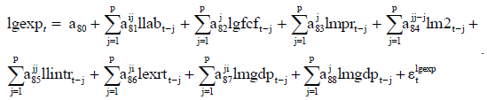
Where α1, α2, α3, α4, α5, α6, α7 are the parameters; t is the time period from 1981:Q1 to 2015:Q4 and et is the stochastic error term. The above equation (2) can be linearized by taking the double log of the equation so as to carry out the several estimation tests and this is shown below:
 (2.1)
(2.1)
Assume that the Nigerian economy is represented by the following structural form:
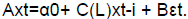 (3)
(3)
Where:
xt is a vector of endogenous variables,
xt-i is a vector of the lagged values of endogenous variables,
εt is a vector of random error of disturbance terms for every variable that captures exogenous factors in the model,
C(L) is a matrix polynomial in the lag operator L of length p,
A is a matrix of n × n dimension, n is the number of variables containing the structural parameters of the contemporaneous endogenous variables, and B is a column vector of dimension n ×1, which contains the contemporaneous response of the variables to the innovations or disturbances [23-28].
There are three steps involved when estimating an SVAR. The first step is to estimate the VAR in its reduced form because the coefficients in the matrices of (3) are unknown, the variables have temporary effects on each other and the model in its current form cannot be identified. To transform (3) into reduced form, we multiply both sides of equation (3) by the inverse of matrix A translating it into a standard VAR representation of:
 (4)
(4)
Further transformation of equation (4) gives:
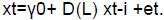 (5)
(5)
Where γ0=A-1α0, D(L)=A-1C(L) and et=A-1Bεt
The focal issue here is to recover the underlying structural disturbances from the estimated VAR. Hence, we can estimate the random stochastic residual A-1Bεt from the residual et of the estimated unrestricted VAR:
 (6)
(6)
Reformulating (6), we have A-1Bεtεt’B’A-1’=etet’ and since etet’=I we have:
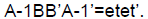 (7)
(7)
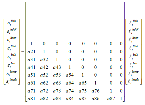
In the second step, we identify the structural model from an estimated VAR. As such, it is necessary to impose restrictions on the structural model. Here, we utilized the nonrecursive method of imposing restrictions in SVARs for the manufacturing sector output component using economic theory as the basic foundation. If there are n variables, equation (5) requires the imposition of n(n+1)/2 restrictions on the 2n2 unknown elements in A and B. Therefore, additional n(3n-1)/2 restrictions are required to be imposed.
 (8)
(8)
From equation (8), it shows that the disturbances or innovations in the reduced form et, are complicated mixtures of the underlying structural shocks, which are not easily interpretable except it is directly linked to the structural shocks. The et is the source of variation in the VAR analysis.
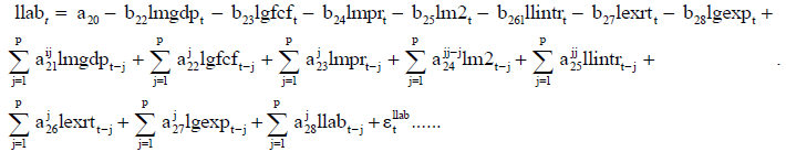
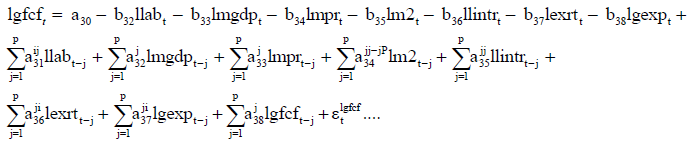
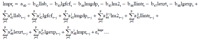
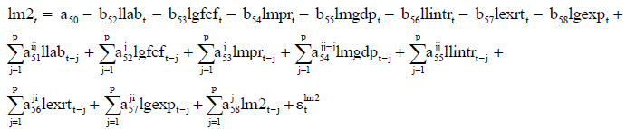
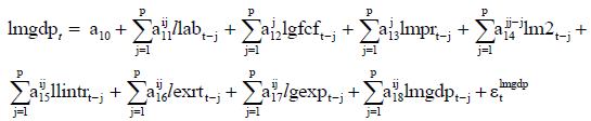
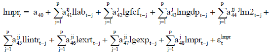
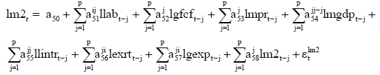
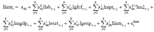
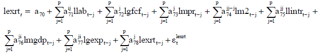
The third step of the SVAR analysis is to use innovation accounting to access the passthrough from the monetary policy and other policy variables to manufacturing sector output. It uses the forecast error et from the estimated reduced form VAR to obtain the impulse response functions (IRF) and forecast error variance decomposition (FEVD), to examine the fractional effects of monetary policy. Equation (3) is called a structural VAR as it is assumed to be determined by some underlying economic theory. Thus the structural model of this study is described by the following dynamic system of simultaneous equations (9-16):
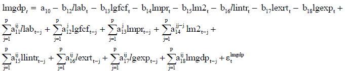 (9)
(9)
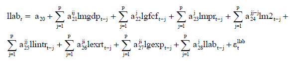
 (10)
(10)
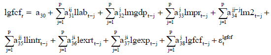
 (11)
(11)
 (12)
(12)
 (13)
(13)
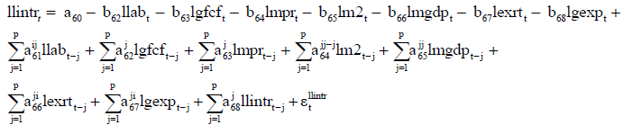 (14)
(14)
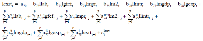 (15)
(15)
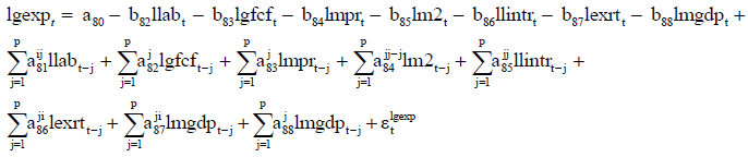 (16)
(16)
The variables: lmgdpt, llabt, lgfcft, lmprt, lm2t, llintt, lexrtt and lgexpt are endogenous
variables. The exogenous error terms:  are independently and identically distributed with mean zero and a constant variance
(σ2). The exogenous error terms may be interpreted as structural innovations. The
realization of each structural innovation is known as capturing unexpected shocks to its
dependent variable respectively, which themselves are uncorrelated with the other
unexpected shocks (εt). In equations (9-16), the endogeneity of lmgdpt, llabt, lgfcft, lmprt,
lm2t, llintt, lexrtt and lgexpt is determined by the values of coefficients, b.
are independently and identically distributed with mean zero and a constant variance
(σ2). The exogenous error terms may be interpreted as structural innovations. The
realization of each structural innovation is known as capturing unexpected shocks to its
dependent variable respectively, which themselves are uncorrelated with the other
unexpected shocks (εt). In equations (9-16), the endogeneity of lmgdpt, llabt, lgfcft, lmprt,
lm2t, llintt, lexrtt and lgexpt is determined by the values of coefficients, b.
The model (9-16) can be re-written in matrix form as follows:
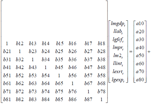
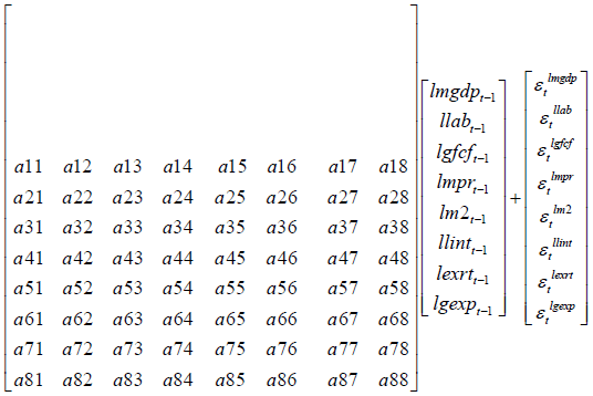
Where j=1, 2, , n.
The reduced form of the VAR model in equation (5) is to be estimated first. This model does not have the instantaneous endogenous variables and is shown in equations (17- 24) as follows:
 (17)
(17)
 (18)
(18)
 (19)
(19)
 (20)
(20)
 (21)
(21)
 (22)
(22)
 (23)
(23)
 (24)
(24)
Without imposing a number of restrictions, the parameters in the SVAR model (9-16) cannot be identified. These restrictions will allow for the contemporaneous interaction between monetary policy variables and manufacturing sector output dynamics of the Nigerian economy.
To impose restrictions, we can use short run SVAR models where current values affect each other (contemporaneous effect), meaning such changes have no long lasting effect; or long run SVAR models where one variable has a long lasting effect in which case, such variable does not return to its initial level. For the short run model, restrictions have to be placed on the A and B matrix, where A matrix is the one for emphasis. The B matrix places restrictions on the error structure.
In analyzing the effects of monetary policy on the manufacturing sector output, an identification scheme for the SVAR is used in the study. The structural shocks in the manufacturing sector output were identified using the non-recursive identification method by placing restriction on the variables in the system as shown in equation (25).
In applying restrictions to each equation, premium was placed on the choice of key economic variables predicated on economic theory and other empirical works.
 (25)
(25)
This first estimation is the selection of the optimal or appropriate lag length. This is necessary in order to check if sufficient lags have been included in the VAR as much lags could lead to a waste of the degrees of freedom while too few lags could result to autocorrelation in the residuals as well as a potential misspecification of the equations. This can be shown in Table 1 where the entire selection criterion (FPE, AIC, HQIC and SBIC) selected two lags.
Table 1: Optimal lag length test.
| Lag | LL | LR | df | p | FPE | AIC | HQIC | SBIC |
|---|---|---|---|---|---|---|---|---|
| 0 | 87.1927 | 4.20E-11 | -1.19989 | -1.12889 | -1.02517 | |||
| 1 | 2020.63 | 3866.9 | 64 | 0.00 | 2.1E-23 | -29.5247 | -28.8857 | -27.9522 |
| 2 | 2229 | 416.73* | 64 | 0.00 | 2.4e-24* | -31.7121* | -30.5051* | -28.7419* |
| 3 | 2257.2 | 56.416 | 64 | 0.739 | 4.20E-24 | 31.1698 | -29.3948 | -26.8019 |
| 4 | 2274.95 | 35.5 | 64 | 0.999 | 8.80E-24 | -30.469 | -28.1261 | -24.7034 |
Sample: 1982q1 - 2014q4, Number of obs=132
Endogenous: llab lgfcf lmpr llint lm2 lexrt lgexp lmgdp
Exogenous: _cons
Source: Authors’ computation using STATA 13
The Augmented Dickey-Fuller test for unit root was used and all variables were found to be non-stationary at levels but were all stationary after the first difference. This can be seen in Table 2.
Table 2: Unit root test results for stationarity of variables.
| Variables | Levels | Remark | First Difference | Remark |
|---|---|---|---|---|
| llab | -0.535 | Non-Stationary | -4.88 | Stationary |
| lgfcf | -1.38 | Non-Stationary | -4.378 | Stationary |
| lmpr | -3.158 | Non-Stationary | -5.697 | Stationary |
| llint | -2.568 | Non-Stationary | -5.187 | Stationary |
| lm2 | -0.793 | Non-Stationary | -3.429 | Stationary |
| lexrt | -1.731 | Non-Stationary | -5.259 | Stationary |
| lgexp | -0.953 | Non-Stationary | -5.98 | Stationary |
| lmgdp | -0.007 | Non-Stationary | -4.892 | Stationary |
| Critical Values | ||||
| 1% | -3.498 | |||
| 5% | -2.888 | |||
| 10% | -2.578 |
Source: Authors’ computation using STATA 13
From Table 3, it can be observed that the entire eigenvalues lie inside the unit circle therefore the VAR satisfies stability condition.
Table 3: Stability test.
| Eigenvalue stability condition | |
|---|---|
| Eigenvalue | Modulus |
| 0.8171972 | 0.817197 |
| .7103723 +.1709321i | 0.730648 |
| .7103723 -.1709321i | 0.730648 |
| .7282052 +.03134427i | 0.728879 |
| .7282052 -.03134427i | 0.728879 |
| 0.6165962 | 0.616596 |
| .4638264 +.01350805i | 0.464023 |
| .4638264 -.01350805i | 0.464023 |
| -.1910868 +.1320135i | 0.232254 |
| -.1910868 +.1320135i | 0.232254 |
| -0.2097935 | 0.209793 |
| -.1786426 +.04098592i | 0.183284 |
| -.1786426 +.04098592i | 0.183284 |
| -.1177171 +.01170538i | 0.118298 |
| -.1177171 +.01170538i | 0.118298 |
| -0.03708589 | 0.037086 |
All the eigenvalues lie inside the unit circle. VAR satisfies stability condition.
Source: Authors’ computation using STATA 13
From Table 4, it can be observed that the prob>chi2 is not statistically significant at 5 percent at lag 1 and 2 hence; we do not reject the null hypothesis of no autocorrelation. Therefore, we conclude that there is no autocorrelation in the residuals.
Table 4: Lagrange-multiplier (LM) test for autocorrelation (Lagrange-multiplier test).
| lag | chi2 | df | prob>chi2 |
|---|---|---|---|
| 1 | 15.2972 | 64 | 1 |
| 2 | 41.7591 | 64 | 0.98589 |
H0: no autocorrelation at lag order
Source: Authors’ computation using STATA 13
Table 5 below shows the contemporaneous relationships among the endogenous variables. It should be noted that these values were estimated in their natural forms at levels so as to prevent any loss of information that may arise as a result of differencing the variables.
Table 5: Estimated coefficients of the short-run variables.
| llab | lgfcf | lmpr | llint | lm2 | lexrt | lgexp | lmgdp | |
|---|---|---|---|---|---|---|---|---|
| llab | 1 | 0 | 0 | 0 | 0 | 0 | 0 | 0 |
| lgfcf | -3.91 | 1 | 0 | 0 | 0 | 0 | 0 | 0 |
| lmpr | -2.97 | 0.56 | 1 | 0 | 0 | 0 | 0 | 0 |
| llint | -3.57 | -0.09 | -0.26 | 1 | 0 | 0 | 0 | 0 |
| lm2 | 0.6 | -0.09 | -0.09 | -0.25 | 1 | 0 | 0 | 0 |
| lexrt | 2.16 | 0.06 | -0.29 | -0.62 | -0.2 | 1 | 0 | 0 |
| lgexp | -0.35 | -0.19 | -0.63 | -0.23 | -0.34 | -0.15 | 1 | 0 |
| lmgdp | -0.08 | -0.17 | -0.05 | 0.31 | 0.06 | -0.01 | -0.12 | 1 |
From Tables 5 and 6, looking at the policy variables, given a positive shock to labour (llab) and capital (lgfcf), the manufacturing contribution to gross domestic product (GDP) (lmgdp) will respond contemporaneously with a marginal decline which is insignificant for labour and significant for capital. On the other hand, given a positive shock in monetary policy rate (lmpr), exchange rate (lexrt) and total government expenditure (lgexp), lmgdp will respond contemporaneously with a marginal decline which is insignificant for lmpr and lexrt and significant for lgexp. Lastly, given a positive shock in lending interest rate and money supply, lmgdp will respond contemporaneously in the same direction although significantly for llint and insignificantly for lm2.
Table 6: Level of significance of estimated coefficients of the short-run variables.
| llab | lgfcf | lmpr | llint | lm2 | lexrt | lgexp | lmgdp | |
|---|---|---|---|---|---|---|---|---|
| llab | 1 | 0 | 0 | 0 | 0 | 0 | 0 | 0 |
| lgfcf | -3.39 | 1 | 0 | 0 | 0 | 0 | 0 | 0 |
| lmpr | -1.8 | 4.73 | 1 | 0 | 0 | 0 | 0 | 0 |
| llint | -4.23 | -1.41 | -5.92 | 1 | 0 | 0 | 0 | 0 |
| lm2 | 1.14 | -2.21 | -3.28 | 5.01 | 1 | 0 | 0 | 0 |
| lexrt | 0.77 | 0.31 | -1.8 | -2.11 | -0.42 | 1 | 0 | 0 |
| lgexp | -0.31 | -2.27 | -9.85 | -1.95 | -1.86 | -4.44 | 1 | 0 |
| lmgdp | -0.12 | -3.21 | -1.02 | 4.15 | 0.51 | -0.41 | -2.24 | 1 |
Source: Authors’ computation using STATA 13
*The above values are the z-values and it must be > 1.98 to be statistically significant.
Impulse Response Functions (IRFs) and Forecast Error Variance Decomposition (FEVD)
The IRFs measure the effects of a shock to an endogenous variable on itself or on another endogenous variable. The impulse response functions show the dynamics of responses of each variable in the model to structural one standard deviation shocks to other variables over time. On the other hand, Forecast error variance decomposition measures the fraction of the forecast error variance of an endogenous variable that can be attributed to orthogonalized shocks to itself or to another endogenous variable. However, given the area of interest of the study, only the impulse response and forecast error variance decomposition of the endogenous variables to the manufacturing contribution to gross domestic product was presented and discussed.

Figure 1: Response of manufacturing contribution to GDP to a shock to monetary policy rate using structural and orthogonalised IRF.
In Figure 1 above, the response of manufacturing contribution to gross domestic product to one standard deviation structural impulse in monetary policy rate is displayed. The manufacturing contribution to gross domestic product increased from the first period to the second period following a one standard deviation structural shock in monetary policy rate but saw a reduction from the third period to the fifth period and then a negative response from the sixth period until it dies out after the eight periods. This negative response of manufacturing contribution to gross domestic product to contractionary monetary policy through the interest rate channel started after the fifth period and this aligns with economic theory.

Figure 2: Response of manufacturing contribution to GDP to a shock to lending interest rate using structural and orthogonalised IRF.
In Figure 2 above, the response of manufacturing contribution to gross domestic product to one standard deviation structural impulse in lending interest rate is displayed. The manufacturing contribution to gross domestic product declined from the first period to the eight periods after which it dies out following a one standard deviation structural shock in the lending interest rate. This is consistent with economic theory where a contractionary monetary policy through the bank lending channel of the credit view under the monetary policy transmission mechanism leads to a decline in output in the economy.

Figure 3: Response of manufacturing contribution to GDP to a shock to money supply using structural and orthogonalised IRF.
In Figure 3 above, the response of manufacturing contribution to gross domestic product to one standard deviation structural impulse in money supply is displayed. The manufacturing contribution to gross domestic product declined in the first period but crossed its steady state value to the positive in period two following a one standard deviation structural shock in the money supply. The positive response of the manufacturing contribution to gross domestic product continued from the second period till it finally disappeared after the eight periods. This is consistent with economic theory after the first period as an expansionary monetary policy through a one standard deviation shock in money supply led to a positive response by the manufacturing contribution to gross domestic product.

Figure 4: Response of manufacturing contribution to GDP to a shock to exchange rate using structural and orthogonalised IRF.
Figure 4 above displays the response of manufacturing contribution to gross domestic product to one standard deviation structural impulse in the exchange rate. Following a one standard deviation structural impulse in the exchange rate, the manufacturing contribution to gross domestic product responded positively from the first period to the fifth period and then negatively in the sixth period before returning to a positive value in the seventh and eight periods after which it dies out. Specifically, the value of the positive response in the manufacturing contribution to gross domestic product was declining from the first period till the sixth period after which it increased in both the seventh and eight periods. This behavior is inconclusive on whether it really aligns with economic theory and from literature; the explanation of the nature of the direction of exchange rate has been difficult. A positive shock in the exchange rate is indicative of a depreciation of the exchange rate which is expected to boost output and make the prices of goods more competitive in the global market on the condition that the economy is productive.

Figure 5: Response of manufacturing contribution to GDP to a shock to total government expenditure using structural and orthogonalised IRF Source: Researcher’s computation using STATA 13.
Figure 5 above displays the response of manufacturing contribution to gross domestic product to one standard deviation structural impulse in the total government expenditure. Following a one standard deviation structural impulse in the total government expenditure, the manufacturing contribution to gross domestic product responded positively after the first and second periods but responded negatively from the third to the eight periods after which it dies out. This does not align with economic theory as an expansionary fiscal policy through an increase in the government expenditure is expected to boost output. The reason for this could be the high proportion of the government expenditure that is spent on recurrent activities rather than capital projects which are intended to boost production in the manufacturing sector.
From the displayed Tables 7 and 8, it can be observed that about 83.67 percent of the variation in the manufacturing contribution to gross domestic product is explained by its own innovation while lending interest rate account for around 7.36 percent. This was the highest relative to other endogenous variables asides manufacturing contribution to gross domestic product. Structural shocks from monetary policy rate, money supply and exchange rate explained about 1.68 percent, 0.11 percent and 0.52 percent respectively of the variation in the manufacturing contribution to gross domestic product. Also, structural innovations in labor force, gross fixed capital formation and total government expenditure accounted for about 0.40 percent, 3.98 percent and 2.29 percent respectively of the variation in the manufacturing contribution to gross domestic product. Hence, examining the fraction of the forecast error variance of manufacturing contribution to gross domestic product that can be attributed to orthogonalized shocks in the various monetary policy transmission mechanisms, one can rank them as follows: credit channel (bank lending channel), interest rate channel, exchange rate channel and money or asset prices channel.
Table 7: Forecast Error Variance Decomposition of Manufacturing Contribution to Gross Domestic Product (MGDP) to shocks in MPR, LINT, M2, EXR, GEXP, LAB, GFCF and MGDP in Nigeria in actual values.
| Period | llab | lgfcf | lmpr | llint | lm2 | lexrt | lgexp | lmgdp |
|---|---|---|---|---|---|---|---|---|
| 1 | 0.000467 | 0.043783 | 0.024399 | 0.092246 | 0.000074 | 0.010072 | 0.029934 | 0.799025 |
| 2 | 0.000437 | 0.040298 | 0.024863 | 0.078371 | 0.000074 | 0.008638 | 0.017044 | 0.830275 |
| 3 | 0.001785 | 0.038739 | 0.022354 | 0.070911 | 0.000038 | 0.006639 | 0.008981 | 0.850553 |
| 4 | 0.003602 | 0.038259 | 0.018449 | 0.067433 | 0.000152 | 0.004908 | 0.006862 | 0.860336 |
| 5 | 0.005252 | 0.038382 | 0.014581 | 0.066676 | 0.000568 | 0.003691 | 0.011091 | 0.85976 |
| 6 | 0.006375 | 0.038836 | 0.011597 | 0.067909 | 0.001349 | 0.002919 | 0.021086 | 0.849929 |
| 7 | 0.006883 | 0.039482 | 0.009664 | 0.070668 | 0.002474 | 0.002422 | 0.0355 | 0.832908 |
| 8 | 0.006879 | 0.040278 | 0.008503 | 0.074612 | 0.003853 | 0.002079 | 0.052663 | 0.811133 |
On the other hand, examining the fraction of the forecast error variance of manufacturing contribution to gross domestic product that can be attributed to orthogonalized shocks in itself and other endogenous variables, one can rank them as follows: manufacturing contribution to gross domestic product (82.16 percent), lending interest rate (7.36 percent), gross fixed capital formation (3.98 percent), total government expenditure (2.29 percent), monetary policy rate (1.68 percent), exchange rate (0.52 percent), labour force (0.40 percent) and money supply (0.11 percent).
Table 8: Forecast Error Variance Decomposition of Manufacturing Contribution to Gross Domestic Product (MGDP) to shocks in MPR, LINT, M2, EXR, GEXP, LAB, GFCF and MGDP in Nigeria in percentage values.
| Period | llab | lgfcf | lmpr | llint | lm2 | lexrt | lgexp | lmgdp |
|---|---|---|---|---|---|---|---|---|
| 1 | 0.05% | 4.38% | 2.44% | 9.22% | 0.01% | 1.01% | 2.99% | 79.90% |
| 2 | 0.04% | 4.03% | 2.49% | 7.84% | 0.01% | 0.86% | 1.70% | 83.03% |
| 3 | 0.18% | 3.87% | 2.24% | 7.09% | 0.00% | 0.66% | 0.90% | 85.06% |
| 4 | 0.36% | 3.83% | 1.84% | 6.74% | 0.02% | 0.49% | 0.69% | 86.03% |
| 5 | 0.53% | 3.84% | 1.46% | 6.67% | 0.06% | 0.37% | 1.11% | 85.98% |
| 6 | 0.64% | 3.88% | 1.16% | 6.79% | 0.13% | 0.29% | 2.11% | 84.99% |
| 7 | 0.69% | 3.95% | 0.97% | 7.07% | 0.25% | 0.24% | 3.55% | 83.29% |
| 8 | 0.69% | 4.03% | 0.85% | 7.46% | 0.39% | 0.21% | 5.27% | 81.11% |
| Total | 3.18% | 31.81% | 13.45% | 58.88% | 0.87% | 4.13% | 18.32% | 669.39% |
| Average | 0.40% | 3.98% | 1.68% | 7.36% | 0.11% | 0.52% | 2.29% | 83.67% |
Source: Authors’ computation using STATA 13
Based on the findings in the study the following recommendations can be given:
1. The monetary authority should ensure that various policies are implemented to guarantee that the lending interest rate to the manufacturing sector is within a single digit, accessible, affordable and sustainable so as to ensure a greater productivity in the sector since it accounted for the biggest variance in the manufacturing contribution to gross domestic product relative to other monetary variables.
2. Central Bank should implement policies to ensure accessibility of the foreign exchange to the manufacturers so as to enable the manufacturing sector obtain inputs such as plant and machineries cheaper from the global market as scarcity makes it more expensive to source for and discourages production.
3. The fiscal authorities specifically the federal government should increase the proportion of the total government expenditure spent on capital expenditure and infrastructural development such as power supply, road networks and rail services in order to ensure that the manufacturing sector operate in a more business friendly environment as well as to bridge the infrastructural gap and improve productivity in the sector.
4. This study recommends that the credit channel through the bank lending channel is the most effective monetary transmission mechanism channel for the manufacturing sector; thus, policy makers as well as those implementing the policies should direct their attention to making the lending interest rate sustainable and affordable to these manufacturers so as to improve output and growth.
5. Lastly, policy synthesis between fiscal and monetary authorities cannot be overemphasized thus; the Central Bank of Nigeria and the Ministry of Finance should always synchronize policies so as to ensure an inclusive and sustainable growth in the manufacturing sector and the Nigerian economy as a whole.
In conclusion, the study examined the effect of monetary policy on the manufacturing sector output in Nigeria using a quarterly data from 1981 to 2015 and employing an eight variable structural vector auto regression model. The variables used in this study are manufacturing contribution to GDP, labor force, gross fixed capital formation, monetary policy rate, lending interest rate, money supply, exchange rate and total government expenditure. The study found out from the impulse response functions that all variables conformed to economic theory except government expenditure. All the monetary variables representing the various monetary channels (interest rate, exchange rate, other assets prices and credit channels) aligned with economic theory. Another major finding of the study was seen in the forecast error variance decomposition, were lending interest rate (7.36 percent) accounted for the biggest variance in the manufacturing sector contribution to gross domestic product while other monetary variables fraction of variances were as follows: monetary policy rate (1.68 percent), exchange rate (0.52 percent) and money supply (0.11 percent).
Copyright © 2025 Research and Reviews, All Rights Reserved